3) Different Guidance Functioning

Florian Berding and Julia Pargmann

2024-01-25

1 Introduction

In this vignette, we would like to show you how the tools of the Iota Concept can be used to analyze the suitability of a coding scheme for rating different kinds of materials. The analysis is very similar to the analysis of different item functioning (DIF) from item-response theory. The focal point here is the question whether or not a coding scheme has the same degree of reliability for different groups of materials. This issue is closely connected to the question if a coding scheme reproduces bias for specific groups.

If a coding scheme is perceived as a measurement instrument, like a test or questionnaire, it must be reliable and valid. Reliability and validity demand the absence of different guidance functioning (DGF), since the existence of DGF means that the data is influenced by other sources, as for example the phenomenon of interest.

We use the term “different guidance functioning” in order to eliminate this kind of analysis from DIF. Furthermore, we would like to express that a coding scheme usually only provides a guideline for raters in assessing a phenomenon.

The analysis of DIF is important for a broad range of applications. For example,

• ensuring that ratings of newspapers do not prefer or discourage specific political parties.
• ensuring that books in different languages are rated without the influence of the different languages.
• ensuring that social media contributions are rated similarly without bias for the platform-specific form of contribution.
• ensuring that material created by different groups of learners is assessed without bias for their socioeconomic background.
• …

In the following, we would like to illustrate this kind of analysis by continuing the example from the first vignette. In order to conduct an analysis of DGF, we need additional data that contains information on how the different coding units are grouped. Let us have a look at the sample data set.

2 Example Analysis

2.1 Basic Analysis

library(iotarelr)
head(iotarelr_written_exams)
#>   Coder A Coder B Coder C    Sex
#> 1 average average    good female
#> 2 average    poor average   male
#> 3    poor average    poor female
#> 4 average average average female
#> 5    poor average    good female
#> 6    poor    poor average female

The data set contains the ratings of exams from three raters and an additional column called “Sex”. This column stores the information if the participant of the exam identifies as male or a female. Since an exam should only measure participants’ performance and should be fair, the Assignment Error Matrix in both groups should not differ. That is, men and women should have the same chance for a good, an average or a poor exam.

The corresponding analysis can be requested via the function check_dgf(). This function is similar to compute_iota2() but has an additional argument, splitcr. This argument uses the group information for the analysis while data only uses the ratings. Please note that calling this function may take some time.

dgf_exam<-check_dgf(data=iotarelr_written_exams[c("Coder A","Coder B","Coder C")],
                    splitcr = iotarelr_written_exams$Sex,
                    random_starts = 300)

The results are stored in the object dgf_exam. For every group specified in the column “Sex”, a model of Iota2 is fitted. The results can be accessed in the same way as with objects created with compute_iota2(). The only thing to do is to request the function get_summary()with the results for the specific group. Let us start with the females.

get_summary(dgf_exam$group_female)
#> Summary
#> 
#> Call: compute_iota2
#> 
#> Number of Raters: 3
#> Number of Categories: 3
#> Categories: average,good,poor
#> Number of Coding Units: 173
#> 
#> Random Start: 300
#> Log-Likelihood: 549.189068930469
#> The best log-likelihood has been replicated.
#> 
#> Primary Parameters
#> Assignment Error Matrix
#>         average  good  poor
#> average   0.887 0.113 0.000
#> good      0.252 0.507 0.241
#> poor      0.441 0.052 0.507
#> 
#> Categorical Sizes
#> average    good    poor 
#>   0.138   0.621   0.241 
#> 
#> Categorical Level
#>           dimensions average   good   poor
#> 1              Alpha  0.8869 0.5069 0.5066
#> 2               Beta   0.382 0.7897 0.5348
#> 3               Iota  0.3061 0.4848 0.3124
#> 4  Iota Error Type I   0.039 0.4716 0.3042
#> 5 Iota Error Type II  0.6549 0.0436 0.3833
#> 
#> Scale Level
#> Iota Index: 0.378
#> Static Iota Index: 0.078
#> Dynamic Iota Index: 0.329

The summary for the females shows the basic information of the fitted model. The best log-likelihood has been replicated. Thus, we can be confident that our model represents the best model for the females.

Special attention should be paid to the Assignment Error Matrix, since this matrix describes how the true categories are assigned. For the females, an average exam is recognized as indeed an average exam in about 88.7% of cases. A good exam is recognized as good exam in about 50% of cases. The remaining 50% of cases are assigned to be an average exam or a a poor exam with the same probability of 25%. A truly poor exam is assigned to be a poor exam in about 50% of cases and an average exam in nearly all other cases. The error to assign a poor exam to be a good exam is only about 5%. Let us now have a look at the results for the men.

get_summary(dgf_exam$group_male)
#> Summary
#> 
#> Call: compute_iota2
#> 
#> Number of Raters: 3
#> Number of Categories: 3
#> Categories: average,good,poor
#> Number of Coding Units: 145
#> 
#> Random Start: 300
#> Log-Likelihood: 461.505161047403
#> The best log-likelihood has not been replicated. Increase the
#>       number of random stars and/or inspect the Assignment Error Matrices and
#>       categorical sizes.
#> 
#> Primary Parameters
#> Assignment Error Matrix
#>         average  good  poor
#> average   0.542 0.262 0.196
#> good      0.333 0.333 0.333
#> poor      0.096 0.163 0.742
#> 
#> Categorical Sizes
#> average    good    poor 
#>   0.593   0.214   0.193 
#> 
#> Categorical Level
#>           dimensions average   good   poor
#> 1              Alpha  0.5416 0.3335 0.7418
#> 2               Beta  0.5334 0.4188 0.5475
#> 3               Iota  0.4704 0.1779 0.3762
#> 4  Iota Error Type I  0.3982 0.3555  0.131
#> 5 Iota Error Type II  0.1314 0.4666 0.4929
#> 
#> Scale Level
#> Iota Index: 0.304
#> Static Iota Index: 0.034
#> Dynamic Iota Index: 0.272

Before we look on the results please note that in some situations it is very difficult to obtain the best estimates. In this example we use 300 random starts and the algorithm is still not able to replicate the solution with the best log-likelihood. Thus, the results for the men can slightly vary for every run.

For the men, the result is very different. According to their Assignment Error Matrix, an average exam is recognized as an average exam only in about 50% of the cases. If it is not recognized as an average exam, it has a higher chance to be considered a good exam than a poor one. Concentrating on the good exams, the Assignment Error Matrix shows the same probability for all categories. This implies that a good exam is assigned randomly to any of the three categories. Only the poor exams have a high chance to be assigned to the correct category with more than 70%.

Comparing the Assignment Error Matrices, it becomes clear that the coding scheme is more reliable for females than for men.

How the different degrees of reliability affect the labeled data can be explored with the function plot_iota(). Here we can directly pass the object dgf_exam to the function.

plot_iota(dgf_exam,
          ylab = "Groups")

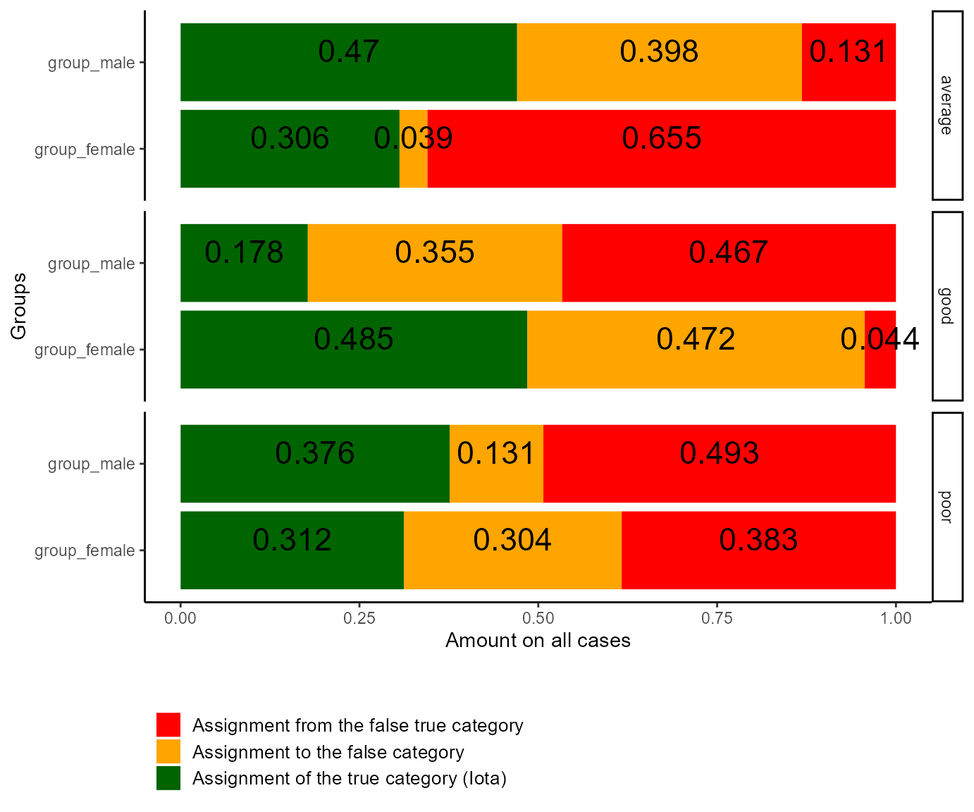
Figure 1: Plot of Iota for different Groups

Let us start with the average exams of the females. The red rectangle for this category implies that the data labeled as “average” contains a lot of exams which truly are either good or poor exams (Iota Error II). The red rectangle is even bigger than the green (Iota) and orange ones (Iota Error I), meaning that the number of averagely good exams is overestimated for the females. Concentrating on the males, the red rectangle (Iota Error II) is quite small but the orange one (Iota Error I) is quite big. Thus, the number of averagely good exams is underestimated.

Regarding the good exams of the females, the red rectangle is quite small (Iota Error II). This means that there is only a small number of average or poor exams that are labeled as good. However, the orange rectangle is quite big (Iota Error I). It nearly has the same size as the green rectangle (Iota). Thus, the data for the good exams misses about half of the corresponding exams. This means that the number of good exams is underestimated in the data set for the females. Concentrating on the males, Iota is only about .18, which is low. Thus, the good exams are not reliably represented in the individual data. In contrast, about 36% of the labeled data are missing good exams (Iota Error I). Instead, the data set is made up of about 46% of exams from other categories (Iota Error II). That is, from truly average or truly poor exams. These exams compensate the missing good exams. As a consequence, in the average of all male participants, the number of good exams is actually quite correct for the males. On the level of single males, the data is not reliable.

Finally, both diagrams for the poor exams look similar for both men and women. For the women, the number of missing poor exams is higher than for the men (Iota Error I). In contrast, the data labeled as poor exams contains more exams which truly belong to the category “good” or “average” for the men as well as for the females (Iota Error II). Thus, in average over all female participants, the number of poor exams is quite correct as well. For the males, the number of poor exams is overestimated. For men as well as for women, the data is not reliable on the individual level.

2.2 Coding Stream Analysis

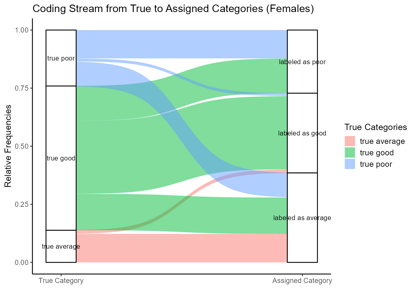
Since version 0.1.3, iotarelr provides an additional analysis of the coding stream that is able to make the interpretation of the data more convenient. This kind of analysis can be request via the function plot_iota2_alluvial(). Please note that the estimates cannot be passed directly to the function. Only the results for a single group are compatible. Applied to the current example, Figure 2 shows the coding stream analysis for the females. The interpretation of the plot is explained in the vignette Get started.

plot_alluvial_females<-plot_iota2_alluvial(
  dgf_exam$group_female,
  label_titel = "Coding Stream from True to Assigned Categories (Females)")
plot(plot_alluvial_females)

Figure 2: Stream Plot for Females

Comparing the boxes for the true and the labeled data, it becomes clear that the number of average exams is overestimated while the number of good exams is underestimated. The sizes of the boxes for the true and assigned poor exams are similar. That is, on average, the number of poor exams is represented in the labeled date quite correctly.

The stream plot illustrates that the exams labeled as good exams are made up by exams which are in truth good exams to a very high extent. This can be seen by the big green curve and the blue and red curves, which in comparison are small. The exams labeled as poor exams are made up of poor and good exams to about 50%. The data labeled as average exams is made up by exams which are in truth good, average and poor to about one third.

plot_alluvial_males<-plot_iota2_alluvial(
  dgf_exam$group_male,
  label_titel = "Coding Stream from True to Assigned Categories (Males)")
plot(plot_alluvial_males)

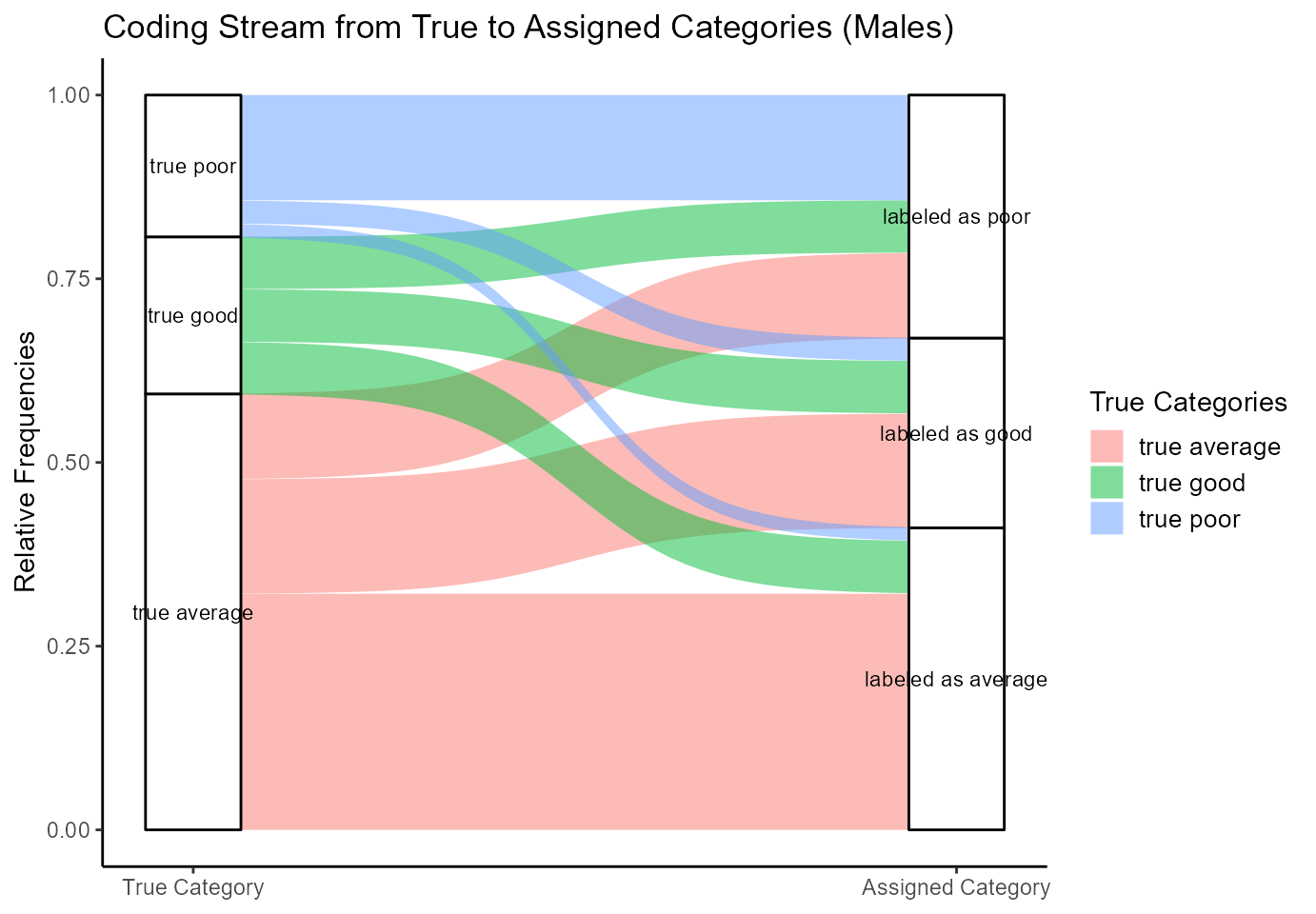
Figure 3: Stream Plot for Males

Turning to the males, the stream plot is very different. Comparing the boxes for the true and assigned categories, it becomes clear that the number of average exams is underestimated while the poor exams are overestimated. Furthermore, the coding scheme leads to a small overestimation of the good exams. Thus, the coding stream plot reflects the results from section 2.1, indicating that the coding scheme tends to divide males’ exams into good or poor exams with no average in between, compared to an error-free measurement.

3 Summary

To sum up, the coding scheme treats the exams of males and females differently. The number of averagely good exams is overestimated for females and underestimated for men. The number of good exams is underestimated for females but quite accurate for men, although the number has its source in the wrong exam categories. Finally, the number of poor exams is quite correct for females, although it sources from quite a lot of wrong exams, while the number of poor exams for the men tends to be overestimated. Thus, in descriptive statistics, females appear to have lower performance than they truly have. For men, the data shows the tendency that they show either a good or a poor performance but nothing in between.

This example shows how the guidance of the coding scheme can be analyzed for different groups of materials. This information can help in developing coding schemes that are free from bias, providing a more reliable and valid source of data for subsequent analysis and conclusions.