5) Test New Raters
Florian Berding and Julia Pargmann
2022-12-22
Source:vignettes/new_rater.Rmd
new_rater.Rmd1 Introduction
Many scientific studies include the development of a new coding scheme for their study which is typically the focus of introductory literature of content analysis (Krippendorff, 2019; Kuckartz, 2018; Mayring, 2015; Schreier, 2012). In these cases, the reliability can be estimated and analyzed as described in the first vignette. In contrast to the literature for new coding schemes, less recommendations refer to the application of existing coding schemes, which are available from published studies or other sources. In these cases, it is not necessary to develop a new scheme, but rather to apply an existing one to new data, often along with new raters. The application of an existing coding scheme to new data has several reasons.
- First, studies using the same coding scheme can be directly compared, contributing to knowledge accumulation in a specific topic or discipline.
- Second, applying an existing coding schemes provides the opportunity to prove the results of prior studies by trying to reproduce them.
- Third, using an existing scheme saves resources, since ideally, the improvement cycle for developing is not necessary. This saves capacities which then become available for other important study characteristics (greater sample sizes, refining specific categories, considering more categories, etc.).
Estimating the reliability of codings based on an existing coding scheme differs from estimating the reliability in the development a coding scheme. The phase of developing a coding scheme aims to provide a theoretically and empirically sound guide for data analysis. This includes that researchers and raters clear up their own interpretation of categories and data and develop the same understanding of the categories based on theory and empirical evidence. Ideally, the final coding scheme is precise enough to document this shared understanding and to guide users to the same interpretation of data and the same assignments of data to categories.
In contrast, the phase of applying an existing coding scheme by new raters does not aim to incorporate the interpretation of data and categories of the new raters. The aim is to train new raters to achieve the understanding of data and categories documented in the scheme. The existing coding scheme represents an already discussed and validated understanding, which new raters have to acquire in order to apply the coding scheme in the same way as in its development study or any other preliminary study. As a consequence, reliability estimation has to consider the existence of a predefined understanding.
2 Estimating the quality of ratings for a new rater
Within the framework of the Iota Concept, this is realized
with the function check_new_rater(). In order to estimate
how well a new rater has developed the understanding documented in a
coding scheme, data and material from existing sources must be used. The
new rater assigns the material to categories and the assignments are
compared to the existing assignments of the material. Based on this
data, the Assignment Error Matrix for the new rater can be
calculated.
To illustrate this process, we continue the example from the first vignette. First, we simulate an “old” study by calculating Iota2 for the example. Second, we calculate the most likely true category for each coding unit. These assignments serve us as “true” categories. In practice, these steps do not have to be performed in every case. If an old source provides the final assignments of coding units, these values can be used as “true” values.
library(iotarelr)
#> Loading required package: ggplot2
#> Warning: package 'ggplot2' was built under R version 4.1.3
#> Loading required package: ggalluvial
#> Warning: package 'ggalluvial' was built under R version 4.1.3
res_iota2<-compute_iota2(data=iotarelr_written_exams[c("Coder A","Coder B","Coder C")],
                         random_starts = 2,
                         trace = FALSE)
expected_categories<-est_expected_categories(
  data=iotarelr_written_exams[c("Coder A","Coder B","Coder C")],
  aem=res_iota2$categorical_level$raw_estimates$assignment_error_matrix)
true_values<-expected_categories$expected_category
Third, a new rater has to rate the same material as the old source.
That is, the new rater has to rate the same exams with the same coding
scheme. Their results are saved in the vector
iotarelr_new_rater. Now, we can request the reliability
estimate for this rater by requesting the function
check_new_rater().
res_new_rater<-check_new_rater(
  true_values = true_values,
  assigned_values = iotarelr_new_rater)
The resulting object is of the class iotarelr_iota2.
Thus, we can use the function get_summary() to look into
the results.
get_summary(res_new_rater)
#> Summary
#>
#> Call: check_new_rater
#>
#> Number of Raters: 1
#> Number of Categories: 3
#> Categories: average,good,poor
#> Number of Coding Units: 318
#>
#> Random Start: NA
#> Log-Likelihood: NA
#>
#>
#> Primary Parameters
#> Assignment Error Matrix
#>         average  good  poor
#> average   0.380 0.239 0.380
#> good      0.167 0.417 0.417
#> poor      0.313 0.178 0.509
#>
#> Categorical Sizes
#> average    good    poor
#>   0.242   0.245   0.513
#>
#> Categorical Level
#>           dimensions average   good   poor
#> 1              Alpha  0.3804 0.4167 0.5092
#> 2               Beta    0.49 0.6287  0.337
#> 3               Iota  0.2078 0.2591 0.3692
#> 4  Iota Error Type I  0.3383 0.3628 0.3559
#> 5 Iota Error Type II  0.4539 0.3781 0.2749
#>
#> Scale Level
#> Iota Index: 0.231
#> Static Iota Index: 0.005
#> Dynamic Iota Index: 0.213
Focusing on the Assignment Error Matrix, the values on the diagonal are very low. This leads to low vales for the Alpha Reliability, which is about 38.04% for average exams, about 41.67% for good exams and about 50.92% for poor exams. Thus, the chance is very high for this new rater to assign the false categories. Please note that the interpretation of these values is now slightly different from the development phase. Here, the high values indicate that the new rater has a high chance to assign different categories to a coding unit as they were assigned in the old study.
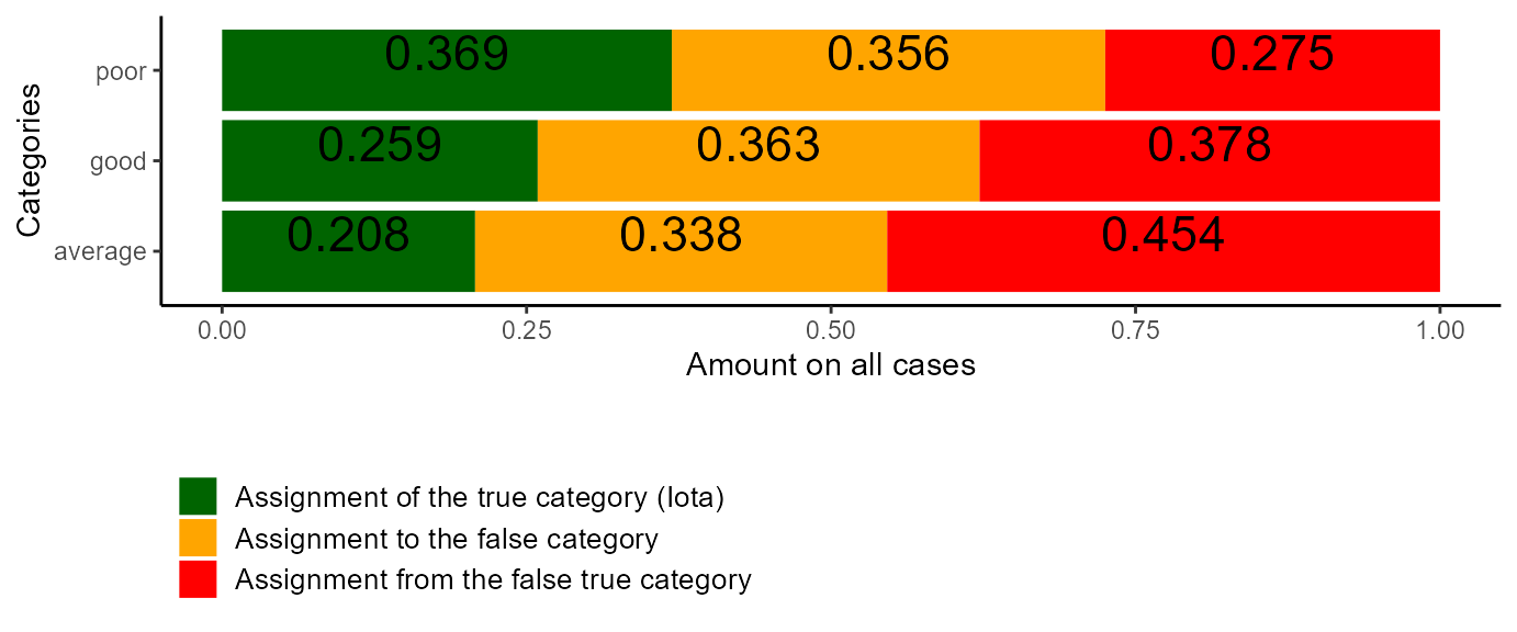
This is also documented in the values for Iota, which range between .2078 for average exams to .3692 for the poor exams. The Dynamic Iota Index is quite low with .213 Finally, we can plot the results for the new rater.
plot_iota(res_new_rater)
Figure 1: Plot of Iota for a New Rater
The plot of Iota for the new rater emphasizes that he is able to recover only a small number of true categories for all kinds of exams. Additionally we can also plot the corresponding coding stream of this new rater.
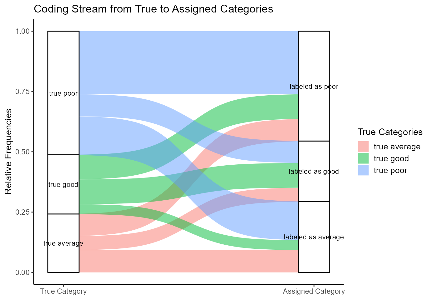
plot_alluvial_new_rater<-plot_iota2_alluvial(res_new_rater)
plot(plot_alluvial_new_rater)
Figure 2: Stream Plot
The boxes on the left side represent how the true categories are distributed in the population. Their height directly reflects the true categorical sizes. The boxes on the right side show the amounts in the labeled data. The curves between the two pairs of boxes illustrate the coding process.
Average exams: Focusing on the true average exams, the plot illustrates that approximately one third of truly average exams are labeled average. This is represented by the big red stream going from true average to labeled as average. The rest of the exams that are truly average is falsely labeled as either poor or good exams. This is shown by the curves going from true average to the respectively labeled category (good or poor). Most of the exams that really are average are not identified as that.
In this alluvial plot, the box for true average exams is slightly smaller than that of the ones labeled as average. That means that the coding scheme tends to overestimate the number of average exams. These false interpretations mostly stem from the true poor category that are labeled as average, shown by the big blue curve going into ‘labeled as average’. In contrast, only a small portion of truly good exams are incorrectly labeled as average, demonstrated by the rather small green curve going from true good to labeled as average.
Good exams: Looking at the good exams, the minority of truly good exams are labeled correctly. This is shown by the green curve going from left (true good exams) to right (labeled as good). Most of the other truly good exams are labeled as poor, which is quite a big difference.
The size of the boxes of the “true good” exams and “the labeled as good” exams is very similar, however the latter is almost entirely made up of the wrong exams. This means that the category seems to have the right size, but truly is not represented correctly because a lot of truly poor and some truly average exams are falsely labeled as good. This can be seen by the bigger blue and smaller red curve going into the box on the right side. In this sense, the coding scheme estimates the number of good exams almost correctly with a slight tendency to overestimate.
Poor exams: Regarding the poor exams, the labeled poor exams box is a little bit smaller than the one for the true poor exams. The composition of these boxes is very different, however. About half of the truly poor exams are labeled correctly, represented by the big blue bar going from left to right. The remainder of the truly poor exams is either labeled as good or average. Most falsely labeled but truly poor exams are labeled average (the bigger blue curve) and some are labeled good (smaller blue curve). Regarding the “labeled as poor” exams on the right, the box is made up of truly poor exams to approximately 50%, with the remainder coming from truly good (the green curve) or average (the red curve) exams. This means that only half of the exams that are truly poor are also recognized as poor.
The box on the left (true poor) and on the right (labeled as poor) have a similar size, although the right one is slightly smaller. This means that the total number of poor exams is estimated quite correct with a slight tendency to underestimate.
3 Conclusion
The function check_new_rater() provides detailed
insights into how a new rater has acquired their understanding of an
existing coding scheme. This information can be used to individually
guide the training process of new raters, since the Assignment Error
Matrix and Iota Reliability provide hints where errors
occur and where everything is fine. This can increase the quality of
codings and saves both costs and time, making the replication and
comparison of studies using content analysis easier.
References
- Früh, W. (2017). Inhaltsanalyse: Theorie und Praxis (9., überarbeitete Auflage). UTB.
- Krippendorff, K. (2019). Content Analysis: An Introduction to Its Methodology (4th Ed.). SAGE.
- Kuckartz, U. (2018). Qualitative Inhaltsanalyse: Methoden, Praxis, Computerunterstützung (4. Auflage). Grundlagentexte Methoden. Beltz.
- Mayring, P. (2015). Qualitative Inhaltsanalyse: Grundlagen und Techniken (12., überarbeitete Auflage). Beltz.
- Schreier, M. (2012). Qualitative Content Analysis in Practice. SAGE.