03 Using R syntax
Florian Berding, Yuliia Tykhonova, Julia Pargmann, Andreas Slopinski, Elisabeth Riebenbauer, Karin Rebmann
Source:vignettes/classification_tasks.Rmd
classification_tasks.Rmd1 Introduction and Overview
1.1 Preface
This vignette introduces the package aifeducation and its usage with R syntax. For users who are unfamiliar with R or those who do not have coding skills in relevant languages (e.g. python), we recommend to start with the graphical user interface AI for Education - Studio which is described in the vignette 02 Using the graphical user interface Aifeducation - Studio.
We assume that aifeducation is installed as described in vignette 01 Get Started. The introduction starts with a brief explanation of basic concepts, which are necessary to work with this package.
1.2 Basic Concepts
In the educational and social sciences, assigning scientific concepts to an observation is an important task that allows researchers to understand an observation, to generate new insights, and to derive recommendations for research and practice.
In educational science, several areas deal with this kind of task. For example, diagnosing students’ characteristics is an important aspect of a teachers’ profession and necessary to understand and promote learning. Another example is the use of learning analytics, where data about students is used to provide learning environments adapted to their individual needs. On another level, educational institutions such as schools and universities can use this information for data-driven performance decisions (Laurusson & White 2014) as well as where and how to improve it. In any case, a real-world observation is aligned with scientific models to use scientific knowledge as a technology for improved learning and instruction.
Supervised machine learning is one concept that allows a link between real-world observations and existing scientific models and theories (Berding et al. 2022). For educational science, this is a great advantage because it allows researchers to use the existing knowledge and insights to apply AI. The drawback of this approach is that the training of AI requires both information about the real world observations and information on the corresponding alignment with scientific models and theories.
A valuable source of data in educational science are written texts, since textual data can be found almost everywhere in the realm of learning and teaching (Berding et al. 2022). For example, teachers often require students to solve a task which they provide in a written form. Students have to create a solution for the tasks which they often document with a short written essay or a presentation. This data can be used to analyze learning and teaching. Teachers’ written tasks for their students may provide insights into the quality of instruction while students’ solutions may provide insights into their learning outcomes and prerequisites.
AI can be a helpful assistant in analyzing textual data since the analysis of textual data is a challenging and time-consuming task for humans.
Please note that an introduction to content analysis, natural language processing or machine learning is beyond the scope of this vignette. If you would like to learn more, please refer to the cited literature.
Before we start, it is necessary to introduce a definition of our understanding of some basic concepts, since applying AI to educational contexts means to combine the knowledge of different scientific disciplines using different, sometimes overlapping, concepts. Even within a single research area, concepts are not unified. Figure 1 illustrates this package’s understanding.
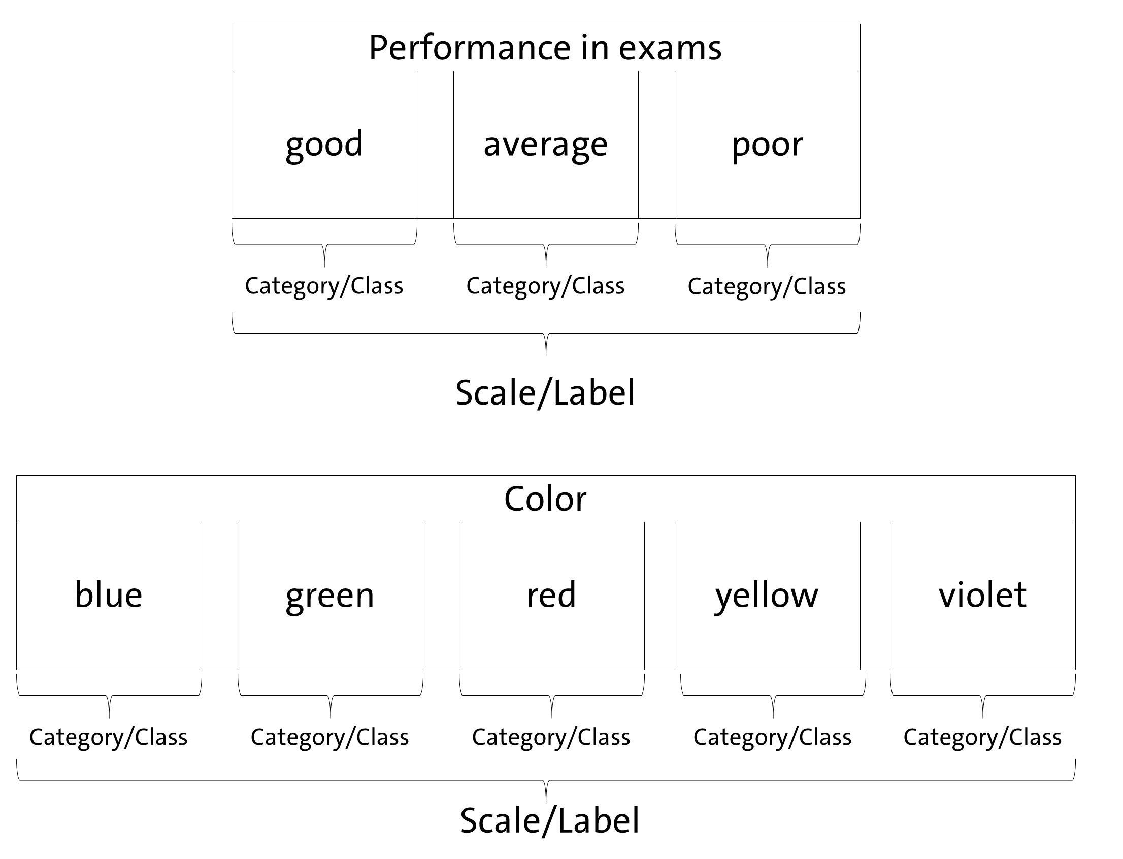
Since aifeducation looks at the application of AI for classification tasks from the perspective of the empirical method of content analysis, there is some overlapping between the concepts of content analysis and machine learning. In content analysis, a phenomenon like performance or colors can be described as a scale/dimension which is made up by several categories (e.g. Schreier 2012, pp. 59). In our example, an exam’s performance (scale/dimension) could be “good”, “average” or “poor”. In terms of colors (scale/dimension) categories could be “blue”, “green”, etc. Machine learning literature uses other words to describe this kind of data. In machine learning, “scale” and “dimension” correspond to the term “label” while “categories” refer to the term “classes” (Chollet, Kalinowski & Allaire 2022, p. 114).
With these clarifications, classification means that a text is assigned to the correct category of a scale or, respectively, that the text is labeled with the correct class. As Figure 2 illustrates, two kinds of data are necessary to train an AI to classify text in line with supervised machine learning principles.
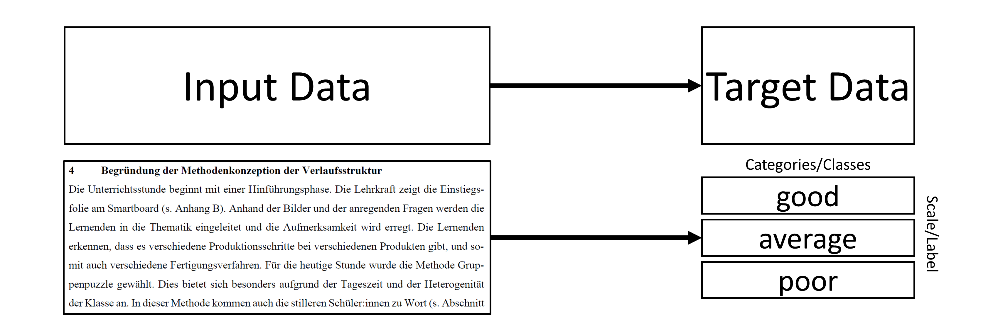
By providing AI with both the textual data as input data and the corresponding information about the class as target data, AI can learn which texts imply a specific class or category. In the above exam example, AI can learn which texts imply a “good”, an “average” or a “poor” judgment. After training, AI can be applied to new texts and predict the most likely class of every new text. The generated class can be used for further statistical analysis or to derive recommendations about learning and teaching.
In use cases as described in this vignette, AI has to “understand” natural language: „Natural language processing is an area of research in computer science and artificial intelligence (AI) concerned with processing natural languages such as English and Mandarin. This processing generally involves translating natural language into data (numbers) that a computer can use to learn about the world. (…)” (Lane , Howard & Hapke 2019, p. 4)
Thus, the first step is to transform raw texts into a a form that is usable for a computer, hence raw texts must be transformed into numbers. In modern approaches, this is usually done through word embeddings. Campesato (2021, p. 102) describes them as “the collective name for a set of language modeling and feature learning techniques (…) where words or phrases from the vocabulary are mapped to vectors of real numbers.” The definition of a word vector is similar: „Word vectors represent the semantic meaning of words as vectors in the context of the training corpus.” (Lane, Howard & Hapke 2019, p. 191). In the next step, the words or text embeddings can be used as input data and the labels as target data when training AI to classify a text.
In aifeducation, these steps are covered with three different types of models, as shown in Figure 3.
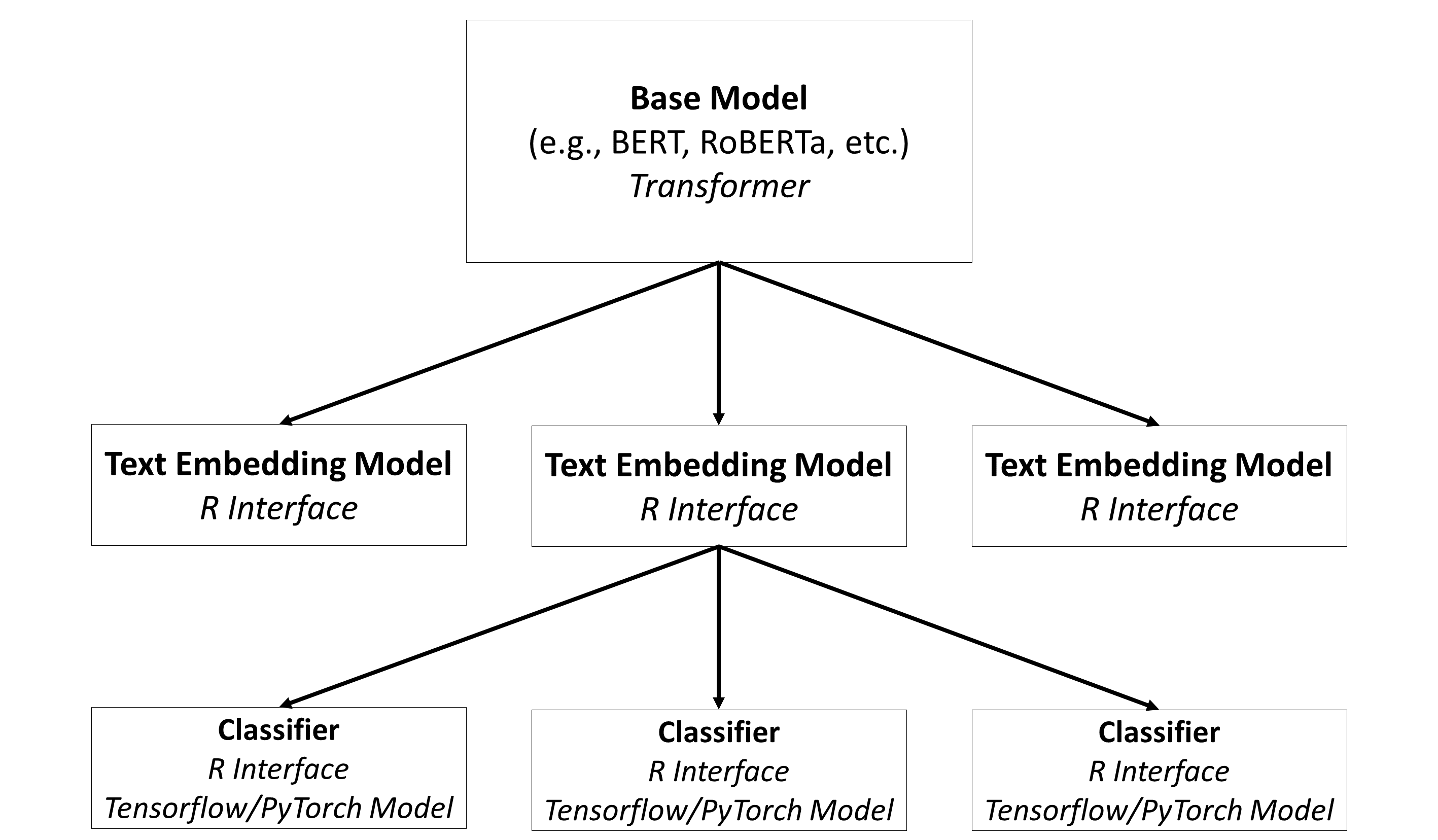
Base Models: The base models contain the capacities to understand natural language. In general, these are transformers such as BERT, RoBERTa, etc. A huge number of pre-trained models can be found on Hugging Face.
Text Embedding Models: The modes are built on top of base models and store directions on how to use these base models for converting raw texts into sequences of numbers. Please note that the same base model can be used to create different text embedding models.
Classifiers: Classifiers are used on top of a text embedding model. They are used to classify a text into categories/classes based on the numeric representation provided by the corresponding text embedding model. Please note that a text embedding model can be used to create different classifiers (e.g. one classifier for colors, one classifier to estimate the quality of a text, etc.).
2 Start Working
2.1 Starting a New Session
Before you can work with aifeducation, you must set up a new
R session. First, you can load aifeducation.
Second, it is necessary that you set up python via ‘reticulate’ and
chose the environment where all necessary python libraries are
available. In case you installed python as suggested in vignette 01 Get started you may start a new session
like this:
library(aifeducation)
prepare_session()
#> Python is already initalized with the virtual environment 'aifeducation'.
#> Try to use this environment.
#> Detected OS: windows
#> Checking python packages. This can take a moment.
#> All necessary python packages are available.
#> python                  : 3.12
#> torch                   : 2.11.0+cu130
#> pyarrow                 : 23.0.1
#> transformers            : 5.8.0
#> tokenizers              : 0.22.2
#> pandas                  : 3.0.2
#> datasets                : 4.8.4
#> calflops                : 0.3.2
#> codecarbon              : 3.2.2
#> safetensors             : 0.7.0
#> torcheval               : 0.0.7
#> accelerate              : 1.13.0
#> numpy                   : 2.4.4
#> GPU Acceleration        : TRUE
#> sentencepiece available : TRUE
#> Version of python package 'transformers' is 5.0.0 or higher. Some older models from hugging face may not work.
#> Load all python objects and functions.
#> Set logger level of python packages.
#> Location for Temporary Files:C:\Users\User\AppData\Local\Temp\RtmpWMhig6/r_aifeducation
Please remember: Every time you start a new session in R, you have to load the library
aifeducationand to configure python. We recommend to use the functionprepare_sessionbecause it performs all necessary steps for setting up python correctly.
Now you can start your work.
2.2 Data Management
2.2.1 Introduction
In the context of use cases for aifeducation, three different types of data are necessary: raw texts, text embeddings, and target data which represent the categories/classes of a text.
To deal with the first two types and to allow the use of large data sets that may not fit into the memory of your machine, the packages ships with two specialized objects.
The first is LargeDataSetForText. Objects of this class
are used to read raw texts from .txt, .pdf, and .xlsx files and store
them for further computations. The second is
LargeDataSetForTextEmbeddings which are used to store the
text embeddings of raw texts which are generated with
TextEmbeddingModels. We will describe the transformation of
raw texts into text embeddings later.
2.2.2 Raw Texts
The creation of a LargeDataSetForText is necessary if
you would like to create or train a base model or to generate text
embeddings. In case you would like to create such a data set for the
first time you have to create an empty data set first:
raw_texts <- LargeDataSetForText$new()To fill this object with raw texts different methods are available depending on the file type you use for storing raw texts.
.txt files
The first alternative is to store raw texts in .txt files. To use these you have to structure your data in a specific way:
- Create a main folder for storing your data.
- Store every raw text/document into a single .txt file into its own folder within the main folder. In every folder there should be only one file for a raw text/document.
- Add an additional .txt file to the folder named
bib_entry.txt. This file contains bibliographic information for the raw text. - Add an additional .txt file to the folder named
license.txtwhich contains a short statement for the license of the text such as “CC BY”. - Add an additional .txt file to the folder named
url_license.txtwhich contains the url/link to the license’s text such as “https://creativecommons.org/licenses/by/4.0/”. - Add an additional .txt file to the folder named
text_license.txtwhich contains the full license in raw texts. - Add an additional .txt file to the folder named
url_source.txtwhich contains the url/link to the text file in the internet.
Applying these rules may result in a data structure as follows:
- Folder “main folder”
- Folder Text A
- text_a.txt
- bib_entry.txt
- license.txt
- url_license.txt
- text_license.txt
- url_source.txt
- Folder Text B
- text_b.txt
- bib_entry.txt
- license.txt
- url_license.txt
- text_license.txt
- url_source.txt
- Folder Text C
- text_C.txt
- bib_entry.txt
- license.txt
- url_license.txt
- text_license.txt
- url_source.txt
- Folder Text A
Now you can call the method add_from_files_txt by
passing the path to the directory of the main folder to
dir_path.
raw_texts$add_from_files_txt(
  dir_path = "main folder",
  clean_text = TRUE
)
The data set will now read all the raw texts in the main folder and
will assign every text the corresponding bib entry, license, etc. Please
note that adding a bib_entry.txt, license.txt,
url_license.txt, text_license.txt, and
url_soruce.text to every folder is optional. If there is no
such file in the corresponding folder, there will be an empty entry in
the data set. However, against the backdrop of the European AI Act, we
recommend to provide both the license and bibliographic information to
make the documentation of your models more straightforward. Furthermore,
some licenses such as those provided by Creative Commons require
statements about the creators, a copyright note, a URL or link to the
source material (if possible), the license of the material and a URL or
link to the license’s text on the internet or the license text itself.
Please check the licenses of the material you are using for the
requirements.
.pdf files
The second alternative is to use .pdf files as a source for raw texts. Here, the necessary structure is similar to .txt files:
- Create a main folder for storing your data.
- Store every raw text/document into a single .pdf file into its own folder within the main folder. In every folder there should be only one file for a raw text/document.
- Add an additional .txt file to the folder named
bib_entry.txt. This file contains bibliographic information for the raw text. - Add an additional .txt file to the folder named
license.txtwhich contains a short statement for the license of the text such as “CC BY”. - Add an additional .txt file to the folder named
url_license.txtwhich contains the URL/link to the license’s text such as “https://creativecommons.org/licenses/by/4.0/”. - Add an additional .txt file to the folder named
text_license.txtwhich contains the full license in raw texts. - Add an additional .txt file to the folder named
url_source.txtwhich contains the url/link to the text file in the internet.
Applying these rules may result in a data structure as follows:
- Folder “main folder”
- Folder Text A
- text_a.pdf
- bib_entry.txt
- license.txt
- url_license.txt
- text_license.txt
- url_source.txt
- Folder Text B
- text_b.pdf
- bib_entry.txt
- license.txt
- url_license.txt
- text_license.txt
- url_source.txt
- Folder Text C
- text_C.pdf
- bib_entry.txt
- license.txt
- url_license.txt
- text_license.txt
- url_source.txt
- Folder Text A
Please not that all files except the text file must be .txt, not .pdf.
Now you can call the method add_from_files_pdf by
passing the path to the directory of the main folder to
dir_path.
raw_texts$add_from_files_pdf(
  dir_path = "main folder",
  clean_text = TRUE
)
As stated above, bib_entry.txt,
license.txt, url_license.txt,
text_license.txt, and url_soruce.text are
optional.
.xlsx files
The third alternative is to store the raw texts into .xlsx files. This alternative is useful if you have many small raw texts. For raw texts that are very large such as books or papers we recommend to store them as .txt or .pdf files.
In order to add raw texts from .xlsx files, the files need a special structure:
- Create a main folder for storing all .xlsx files you would like to read.
- All .xlsx files must contain the names of the columns in the first row and the names must be identical for each column across all .xslx files you would like to read.
- Every .xslx files must contain a column storing the text ID and must contain a column storing the raw text. Every text must have a unique ID across all .xlsx files.
- Every .xslx file can contain an additional column for the bib entry.
- Every .xslx file can contain an additional column for the license.
- Every .xslx file can contain an additional column for the license’s URL.
- Every .xslx file can contain an additional column for the license’s text.
- Every .xslx file can contain an additional column for the source’s URL.
Your .xlsx file may look like
| id | text | bib | license | url_license | text_license | url_source |
|---|---|---|---|---|---|---|
| z3 | This is an example. | Author (2019) | CC BY | Example URL | Text | Example URL |
| a3 | This is a second example. | Author (2022) | CC BY | Example URL | Text | Example URL |
| … | … | … | … |
Now you can call the method add_from_files_xlsx by
passing the path to the directory of the main folder to
dir_path. Please do not forget to specify the column names
for ID and text as well as for the other columns.
raw_texts$add_from_files_xlsx(
  dir_path = "main folder",
  id_column = "id",
  text_column = "text",
  bib_entry_column = "bib_entry",
  license_column = "license",
  url_license_column = "url_license",
  text_license_column = "text_license",
  url_source_column = "url_source"
)
Cleant text
For .txt and .pdf files you can set the argument
clean_text=TRUE. This requests an algorithm that should
pre-process the raw texts and applies the following modifications:
- Some special symbols are removed.
- All spaces at the beginning and the end of a row are removed.
- Multiple spaces are reduced to single space.
- All rows with a number from 1 to 999 at the beginning or at the end are removed (header and footer).
- List of content is removed.
- Hyphenation is made undone.
- Line breaks within a paragraph are removed.
- Multiple line breaks are reduced to a single line break.
The aim of these changes is to provide a clean plain text in order to increase the performance and quality of all analyses.
IDs In case of .xlsx files, the texts’ IDs are set to the IDs stored in the corresponding column for ID. In case of .pdf and .txt files, the file names are used as ID (without the file extension).
Please note that a consequence of this is that two files text_01.txt and text_01.pdf have the same ID, which is not allowed. Please ensure that you use unique IDs across file formats.
Saving and loading a data set
Once you have create a LargeDataSetForText you can save
your data to disk by calling the function save_to_disk. In
our example the code would be:
save_to_disk(
  object = raw_texts,
  dir_path = "examples",
  folder_name = "raw_texts"
)
The argument object requires the object you would like
to save. In our case this is raw_texts. With
dir_path you specific the location where to save the object
and with folder_name you define the name of the folder that
will be created within that directory. In this folder the data set is
saved.
To load an existing data set, you can call the function
load_from_disk with the directory path where you stored the
data. In our case this would be:
raw_text_dataset <- load_from_disk("examples/raw_texts")Now you can work with your data.
2.2.3 Text Embeddings
The numerical representations of raw texts (called text embeddings)
are stored with objects of class
LargeDataSetForTextEmbeddings. These kinds of data sets are
generated by some models such as TextEmbeddingModels. Thus,
you will never need to create such a data set manually.
However, you will need this kind of data set to train a classifier or
to predict the categories/classes of raw texts. Thus, it may be
advantageous to save already transformed data. You can save and load an
object of this class with the functions save_to_disk and
load_from_disk.
Let us assume that we have a
LargeDataSetForTextEmbeddings called
text_embeddings. Saving this object may look like:
save_to_disk(
  object = text_embeddings,
  dir_path = "examples",
  folder_name = "text_embeddings"
)
The data set will be saved at examples/text_embeddings.
Loading this data set may look like:
new_text_embeddings <- load_from_disk("examples/text_embeddings")2.2.4 Target Data
The last data type necessary for working with
aifeducation are the categories/classes of given raw texts.
For this kind of data we currently do not provide a special object. You
just need a named factor storing the
classes/categories for a dimension. It is also important that the names
equal the ID of the corresponding raw texts/text embeddings since
matching the classes/categories to texts is done with the help of these
names.
Saving and loading can be done with R’s functions
save and load.
2.3 Example Data for this Vignette
To illustrate the steps in this vignette, we cannot use data from
educational settings since these data is generally protected by privacy
policies. Therefore, we use a subset of the Standford Movie Review
Dataset provided by Maas et al. (2011) which is part of the package. You
can access the data set with imdb_movie_reviews.
We now have a data set with three columns. The first column contains the raw text, the second contains the rating of the movie (positive or negative), and the third column the ID of the movie review. About 200 reviews imply a positive rating of a movie and about 100 imply a negative rating.
For this tutorial, we modify this data set by setting about 50
positive and 25 negative reviews to NA, indicating that
these reviews are not labeled.
example_data <- imdb_movie_reviews
example_data$label <- as.character(example_data$label)
example_data$label[c(76:100)] <- NA
example_data$label[c(201:250)] <- NA
table(example_data$label)
#>
#> neg pos
#>  75 150
We will now create a LargeDataSetForText from this
data.frame. Before we can do this we must ensure that the
data.set has all necessary columns:
colnames(example_data)
#> [1] "text"  "label" "id"
Now we have to add two columns. For this tutorial we do not add any bibliographic or license information although this is recommended in practice.
example_data$bib_entry <- NA
example_data$license <- NA
colnames(example_data)
#> [1] "text"      "label"     "id"        "bib_entry" "license"
Now the data.frame is ready as input for our data set.
The “label” column will not be included.
data_set_reviews_text <- LargeDataSetForText$new()
data_set_reviews_text$add_from_data.frame(example_data)
You can inspect the data set with print.
print(data_set_reviews_text)
#> Object : LargeDataSetForText
#> Columns: id, text, bib_entry, license, url_license, text_license, url_source
#> Rows   : 300
We save the categories/labels within a separate factor.
We will now use this data to show you how to use the different objects and functions in aifeducation.
3 Base Models
3.1 Overview
Base models are the foundation of all further models in aifeducation. At the moment, these are transformer models such modernBERT (Warner et al. 2024), MPNet (Song et al. 2020), BERT (Devlin et al. 2019), RoBERTa (Liu et al. 2019), and Funnel-Transformer (Dai et al. 2020). In general, these models are trained on a large corpus of general texts in the first step. In the next step, the models are fine-tuned to domain-specific texts and/or fine-tuned for specific tasks. Since the creation of base models requires a huge number of texts resulting in high computational time, it is recommended to use pre-trained models. These can be found on Hugging Face. Sometimes, however, it is more straightforward to create a new model to fit a specific purpose. aifeducation supports the option to both create and train/fine-tune base models.
In this chapter we concentrate on creating a new model. The usage of a pre-trained model from Hugging Face is described in chapter 4.
Every transformer model is composed of two parts:
- the tokenizer which splits raw texts into smaller pieces to model a large number of words with a limited, small number of tokens and
- the neural network that is used to model the capabilities for understanding natural language.
3.2 Creation of a Tokenizer
The first stept is to set up a tokenizer.
In aifeducation you can choose between different models. In
this example we use a WordPieceTokenizer. To create a new one we first
call the method new.
tokenizer <- WordPieceTokenizer$new()Now we have an empty tokenizer which we can configure by calling the
corresponding method. The available parameter depend on the kind of
tokenizer. In the case of a WordPieceTokenizer we have only two options.
The first, vocab_size determines how many tokens the
tokenizer should know. The second determines if all words should be
transformed to lower case before tokenization. since we use only a very
small data set for illustrating the usage of the package we set
vocab_size = 200. In real case applications this value
should be larger. You can find more information on this topic in
vignette 04 Model configuration and
training.
tokenizer$configure(
  vocab_size = 200,
  vocab_do_lower_case = FALSE
)
In the next step we have to train the model by calling the method
train. Here we pass a dataset for text to the parameter
text_dataset. This raw text is used to train the model.
In addition, we can set up sustainability tracking of this process to
estimate its ecological impact with help of the python library
codecarbon. Thus, sustain_track is set to
TRUE by default. If you use the sustainability tracker you
must provide the alpha-3 code for the country where your computer is
located (e.g., “CAN”=“Canada”, “DEU”=“Germany”). A list with the codes
can be found on Wikipedia.
The reason is that different countries use different sources and
techniques for generating their energy resulting in a specific impact on
CO2 emissions. For the USA and Canada you can additionally specify a
region by setting sustain_region. Please refer to the
documentation of codecarbon for more information.
tokenizer$train(
  text_dataset = data_set_reviews_text,
  statistics_max_tokens_length = 512,
  sustain_track = TRUE,
  sustain_iso_code = "DEU",
  sustain_region = NULL,
  sustain_interval = 15,
  sustain_log_level = "error",
  trace = TRUE
)
#> 2026-07-06 11:35:06 Start Sustainability Tracking
#> 2026-07-06 11:35:09 Stop Sustainability Tracking
Training a tokenizer is a very fast process. Thus, even for a huge number of texts the computations should take only some minutes.
Now the model is ready to use. At the beginning we can explore some tokenizer statistics.
# We use t() to improve the readability of the table
t(tokenizer$get_tokenizer_statistics())
#>                   [,1]
#> step              "creation"
#> date              "2026-07-06 11:35:09"
#> max_tokens_length "512"
#> n_sequences       "653"
#> n_words           "90195"
#> n_tokens          "257269"
#> mu_t              "393.9801"
#> mu_w              "138.124"
#> mu_g              "2.852364"
In this table you can see an estimation of the number of words for the whole training data set, the total number of tokens resulting from the raw texts and the number of sequences if the length of a sequence is limited to the value shown in the column ‘max_token_length’. Furthermore, you can see the three statistics proposed by Kaya and Tantug (2024, p.5). \mu_t refers to the average number of tokens per sequence, \mu_w refers to the average number of words per sequence, and \mu_g refers to the average number of tokens per word. \mu_g is called the tokenizer granularity rate and describes how many tokens are necessary to represent a single word. This value is very important as a higher value implies that the same text is spitted into a longer sequence of tokens than for a tokenizer with a lower value. Since large language models have a maximum limit on the length of a token sequence this value has in impact on how many words of a text can be processed by a base model.
If you would like to see how the tokenizer works you can call the method ‘encode’.
tokenizer$encode(
  raw_text = "This is a good movie.",
  token_encodings_only = TRUE,
  token_to_int = FALSE
)
#> [[1]]
#> [[1]][[1]]
#>   [1] "[CLS]" "T"     "##h"   "##is"  "is"    "a"     "g"     "##o"   "##o"
#>  [10] "##d"   "m"     "##o"   "##v"   "##i"   "##e"   "."     "[SEP]" "[PAD]"
#>  [19] "[PAD]" "[PAD]" "[PAD]" "[PAD]" "[PAD]" "[PAD]" "[PAD]" "[PAD]" "[PAD]"
#>  [28] "[PAD]" "[PAD]" "[PAD]" "[PAD]" "[PAD]" "[PAD]" "[PAD]" "[PAD]" "[PAD]"
#>  [37] "[PAD]" "[PAD]" "[PAD]" "[PAD]" "[PAD]" "[PAD]" "[PAD]" "[PAD]" "[PAD]"
#>  [46] "[PAD]" "[PAD]" "[PAD]" "[PAD]" "[PAD]" "[PAD]" "[PAD]" "[PAD]" "[PAD]"
#>  [55] "[PAD]" "[PAD]" "[PAD]" "[PAD]" "[PAD]" "[PAD]" "[PAD]" "[PAD]" "[PAD]"
#>  [64] "[PAD]" "[PAD]" "[PAD]" "[PAD]" "[PAD]" "[PAD]" "[PAD]" "[PAD]" "[PAD]"
#>  [73] "[PAD]" "[PAD]" "[PAD]" "[PAD]" "[PAD]" "[PAD]" "[PAD]" "[PAD]" "[PAD]"
#>  [82] "[PAD]" "[PAD]" "[PAD]" "[PAD]" "[PAD]" "[PAD]" "[PAD]" "[PAD]" "[PAD]"
#>  [91] "[PAD]" "[PAD]" "[PAD]" "[PAD]" "[PAD]" "[PAD]" "[PAD]" "[PAD]" "[PAD]"
#> [100] "[PAD]" "[PAD]" "[PAD]" "[PAD]" "[PAD]" "[PAD]" "[PAD]" "[PAD]" "[PAD]"
#> [109] "[PAD]" "[PAD]" "[PAD]" "[PAD]" "[PAD]" "[PAD]" "[PAD]" "[PAD]" "[PAD]"
#> [118] "[PAD]" "[PAD]" "[PAD]" "[PAD]" "[PAD]" "[PAD]" "[PAD]" "[PAD]" "[PAD]"
#> [127] "[PAD]" "[PAD]" "[PAD]" "[PAD]" "[PAD]" "[PAD]" "[PAD]" "[PAD]" "[PAD]"
#> [136] "[PAD]" "[PAD]" "[PAD]" "[PAD]" "[PAD]" "[PAD]" "[PAD]" "[PAD]" "[PAD]"
#> [145] "[PAD]" "[PAD]" "[PAD]" "[PAD]" "[PAD]" "[PAD]" "[PAD]" "[PAD]" "[PAD]"
#> [154] "[PAD]" "[PAD]" "[PAD]" "[PAD]" "[PAD]" "[PAD]" "[PAD]" "[PAD]" "[PAD]"
#> [163] "[PAD]" "[PAD]" "[PAD]" "[PAD]" "[PAD]" "[PAD]" "[PAD]" "[PAD]" "[PAD]"
#> [172] "[PAD]" "[PAD]" "[PAD]" "[PAD]" "[PAD]" "[PAD]" "[PAD]" "[PAD]" "[PAD]"
#> [181] "[PAD]" "[PAD]" "[PAD]" "[PAD]" "[PAD]" "[PAD]" "[PAD]" "[PAD]" "[PAD]"
#> [190] "[PAD]" "[PAD]" "[PAD]" "[PAD]" "[PAD]" "[PAD]" "[PAD]" "[PAD]" "[PAD]"
#> [199] "[PAD]" "[PAD]" "[PAD]" "[PAD]" "[PAD]" "[PAD]" "[PAD]" "[PAD]" "[PAD]"
#> [208] "[PAD]" "[PAD]" "[PAD]" "[PAD]" "[PAD]" "[PAD]" "[PAD]" "[PAD]" "[PAD]"
#> [217] "[PAD]" "[PAD]" "[PAD]" "[PAD]" "[PAD]" "[PAD]" "[PAD]" "[PAD]" "[PAD]"
#> [226] "[PAD]" "[PAD]" "[PAD]" "[PAD]" "[PAD]" "[PAD]" "[PAD]" "[PAD]" "[PAD]"
#> [235] "[PAD]" "[PAD]" "[PAD]" "[PAD]" "[PAD]" "[PAD]" "[PAD]" "[PAD]" "[PAD]"
#> [244] "[PAD]" "[PAD]" "[PAD]" "[PAD]" "[PAD]" "[PAD]" "[PAD]" "[PAD]" "[PAD]"
#> [253] "[PAD]" "[PAD]" "[PAD]" "[PAD]" "[PAD]" "[PAD]" "[PAD]" "[PAD]" "[PAD]"
#> [262] "[PAD]" "[PAD]" "[PAD]" "[PAD]" "[PAD]" "[PAD]" "[PAD]" "[PAD]" "[PAD]"
#> [271] "[PAD]" "[PAD]" "[PAD]" "[PAD]" "[PAD]" "[PAD]" "[PAD]" "[PAD]" "[PAD]"
#> [280] "[PAD]" "[PAD]" "[PAD]" "[PAD]" "[PAD]" "[PAD]" "[PAD]" "[PAD]" "[PAD]"
#> [289] "[PAD]" "[PAD]" "[PAD]" "[PAD]" "[PAD]" "[PAD]" "[PAD]" "[PAD]" "[PAD]"
#> [298] "[PAD]" "[PAD]" "[PAD]" "[PAD]" "[PAD]" "[PAD]" "[PAD]" "[PAD]" "[PAD]"
#> [307] "[PAD]" "[PAD]" "[PAD]" "[PAD]" "[PAD]" "[PAD]" "[PAD]" "[PAD]" "[PAD]"
#> [316] "[PAD]" "[PAD]" "[PAD]" "[PAD]" "[PAD]" "[PAD]" "[PAD]" "[PAD]" "[PAD]"
#> [325] "[PAD]" "[PAD]" "[PAD]" "[PAD]" "[PAD]" "[PAD]" "[PAD]" "[PAD]" "[PAD]"
#> [334] "[PAD]" "[PAD]" "[PAD]" "[PAD]" "[PAD]" "[PAD]" "[PAD]" "[PAD]" "[PAD]"
#> [343] "[PAD]" "[PAD]" "[PAD]" "[PAD]" "[PAD]" "[PAD]" "[PAD]" "[PAD]" "[PAD]"
#> [352] "[PAD]" "[PAD]" "[PAD]" "[PAD]" "[PAD]" "[PAD]" "[PAD]" "[PAD]" "[PAD]"
#> [361] "[PAD]" "[PAD]" "[PAD]" "[PAD]" "[PAD]" "[PAD]" "[PAD]" "[PAD]" "[PAD]"
#> [370] "[PAD]" "[PAD]" "[PAD]" "[PAD]" "[PAD]" "[PAD]" "[PAD]" "[PAD]" "[PAD]"
#> [379] "[PAD]" "[PAD]" "[PAD]" "[PAD]" "[PAD]" "[PAD]" "[PAD]" "[PAD]" "[PAD]"
#> [388] "[PAD]" "[PAD]" "[PAD]" "[PAD]" "[PAD]" "[PAD]" "[PAD]" "[PAD]" "[PAD]"
#> [397] "[PAD]" "[PAD]" "[PAD]" "[PAD]" "[PAD]" "[PAD]" "[PAD]" "[PAD]" "[PAD]"
#> [406] "[PAD]" "[PAD]" "[PAD]" "[PAD]" "[PAD]" "[PAD]" "[PAD]" "[PAD]" "[PAD]"
#> [415] "[PAD]" "[PAD]" "[PAD]" "[PAD]" "[PAD]" "[PAD]" "[PAD]" "[PAD]" "[PAD]"
#> [424] "[PAD]" "[PAD]" "[PAD]" "[PAD]" "[PAD]" "[PAD]" "[PAD]" "[PAD]" "[PAD]"
#> [433] "[PAD]" "[PAD]" "[PAD]" "[PAD]" "[PAD]" "[PAD]" "[PAD]" "[PAD]" "[PAD]"
#> [442] "[PAD]" "[PAD]" "[PAD]" "[PAD]" "[PAD]" "[PAD]" "[PAD]" "[PAD]" "[PAD]"
#> [451] "[PAD]" "[PAD]" "[PAD]" "[PAD]" "[PAD]" "[PAD]" "[PAD]" "[PAD]" "[PAD]"
#> [460] "[PAD]" "[PAD]" "[PAD]" "[PAD]" "[PAD]" "[PAD]" "[PAD]" "[PAD]" "[PAD]"
#> [469] "[PAD]" "[PAD]" "[PAD]" "[PAD]" "[PAD]" "[PAD]" "[PAD]" "[PAD]" "[PAD]"
#> [478] "[PAD]" "[PAD]" "[PAD]" "[PAD]" "[PAD]" "[PAD]" "[PAD]" "[PAD]" "[PAD]"
#> [487] "[PAD]" "[PAD]" "[PAD]" "[PAD]" "[PAD]" "[PAD]" "[PAD]" "[PAD]" "[PAD]"
#> [496] "[PAD]" "[PAD]" "[PAD]" "[PAD]" "[PAD]" "[PAD]" "[PAD]" "[PAD]" "[PAD]"
#> [505] "[PAD]" "[PAD]" "[PAD]" "[PAD]" "[PAD]" "[PAD]" "[PAD]" "[PAD]"
Here you can see that the tokenizer split the words into several tokens and adds some special tokens.
tokenizer$encode(
  raw_text = "This is a good movie.",
  token_encodings_only = TRUE,
  token_to_int = TRUE
)
#> [[1]]
#> [[1]][[1]]
#>   [1]   0  53 112 174 188  61  67 111 111 104  73 111 123 102  97  17   1   3
#>  [19]   3   3   3   3   3   3   3   3   3   3   3   3   3   3   3   3   3   3
#>  [37]   3   3   3   3   3   3   3   3   3   3   3   3   3   3   3   3   3   3
#>  [55]   3   3   3   3   3   3   3   3   3   3   3   3   3   3   3   3   3   3
#>  [73]   3   3   3   3   3   3   3   3   3   3   3   3   3   3   3   3   3   3
#>  [91]   3   3   3   3   3   3   3   3   3   3   3   3   3   3   3   3   3   3
#> [109]   3   3   3   3   3   3   3   3   3   3   3   3   3   3   3   3   3   3
#> [127]   3   3   3   3   3   3   3   3   3   3   3   3   3   3   3   3   3   3
#> [145]   3   3   3   3   3   3   3   3   3   3   3   3   3   3   3   3   3   3
#> [163]   3   3   3   3   3   3   3   3   3   3   3   3   3   3   3   3   3   3
#> [181]   3   3   3   3   3   3   3   3   3   3   3   3   3   3   3   3   3   3
#> [199]   3   3   3   3   3   3   3   3   3   3   3   3   3   3   3   3   3   3
#> [217]   3   3   3   3   3   3   3   3   3   3   3   3   3   3   3   3   3   3
#> [235]   3   3   3   3   3   3   3   3   3   3   3   3   3   3   3   3   3   3
#> [253]   3   3   3   3   3   3   3   3   3   3   3   3   3   3   3   3   3   3
#> [271]   3   3   3   3   3   3   3   3   3   3   3   3   3   3   3   3   3   3
#> [289]   3   3   3   3   3   3   3   3   3   3   3   3   3   3   3   3   3   3
#> [307]   3   3   3   3   3   3   3   3   3   3   3   3   3   3   3   3   3   3
#> [325]   3   3   3   3   3   3   3   3   3   3   3   3   3   3   3   3   3   3
#> [343]   3   3   3   3   3   3   3   3   3   3   3   3   3   3   3   3   3   3
#> [361]   3   3   3   3   3   3   3   3   3   3   3   3   3   3   3   3   3   3
#> [379]   3   3   3   3   3   3   3   3   3   3   3   3   3   3   3   3   3   3
#> [397]   3   3   3   3   3   3   3   3   3   3   3   3   3   3   3   3   3   3
#> [415]   3   3   3   3   3   3   3   3   3   3   3   3   3   3   3   3   3   3
#> [433]   3   3   3   3   3   3   3   3   3   3   3   3   3   3   3   3   3   3
#> [451]   3   3   3   3   3   3   3   3   3   3   3   3   3   3   3   3   3   3
#> [469]   3   3   3   3   3   3   3   3   3   3   3   3   3   3   3   3   3   3
#> [487]   3   3   3   3   3   3   3   3   3   3   3   3   3   3   3   3   3   3
#> [505]   3   3   3   3   3   3   3   3
If you change the parameter token_to_int = TRUE you
receive the same result but instead of the tokens you get the index of
the token in the tokenizer’s vocabulary. For example the id 0 refers to
the token [CLS] in this example.
In the case you have a sequence of id and would like to know which
tokens belong to these numbers you can call the method
decode.
tokenizer$decode(
  int_seqence = list(list(c(0, 53, 109, 174, 188, 61, 67, 97, 97, 112, 73, 97, 110, 99, 101, 17, 1))),
  to_token = TRUE
)
#> [[1]]
#> [[1]][[1]]
#> [1] "[CLS] T ##g ##is is a g ##e ##e ##h m ##e ##z ##t ##y . [SEP]"
If you would like to analyse the ecological impact of training the tokenizer you can get an estimation of energy consumption and CO2-emission.
# We use t() to improve the readability of the table
t(tokenizer$get_sustainability_data("training"))
#>                                      [,1]
#> sustainability_tracked               "TRUE"
#> date                                 "2026-07-06 11:35:09"
#> task                                 "Create tokenizer"
#> sustainability_data.duration_sec     "1.420916"
#> sustainability_data.co2eq_kg         "9.974007e-06"
#> sustainability_data.cpu_energy_kwh   "1.675727e-05"
#> sustainability_data.gpu_energy_kwh   "5.482227e-06"
#> sustainability_data.ram_energy_kwh   "3.942436e-06"
#> sustainability_data.total_energy_kwh "2.618193e-05"
#> technical.tracker                    "codecarbon"
#> technical.py_package_version         "3.2.2"
#> technical.cpu_count                  "12"
#> technical.cpu_model                  "12th Gen Intel(R) Core(TM) i5-12400F"
#> technical.gpu_count                  "1"
#> technical.gpu_model                  "1 x NVIDIA GeForce RTX 4070"
#> technical.ram_total_size             "15.84258"
#> region.country_name                  "Germany"
#> region.country_iso_code              "DEU"
#> region.region                        NA
Since tokenizers can be trained very efficient these values will be very low in most cases.
Finally, you can save and load your model. This is done for all
object with the function pair save_to_disk and
load_from_disk.
save_to_disk(
  object = tokenizer,
  dir_path = "examples",
  folder_name = "example_tokenizer"
)
tokenizer <- load_from_disk("examples/example_tokenizer")To get a short summary of a tokenizer you can use
print.
print(tokenizer)
#> Object     : WordPieceTokenizer
#> Configured : TRUE
#> Trained    : TRUE
#> Vocab Size : 200
#> Tokens/Word: 2.85236432174733
#> Mask Token : [MASK]
#> Pad Token  : [PAD]
#> Unk Token  : [UNK]
Now you are ready to create a base model.
3.3 Creating a BaseModel
At the beginning you can choose between the different supported
transformer architectures. Depending on the architecture, you have
different options determining the shape of your neural network. For this
vignette we use a BERT (Devlin et al. 2019) model which can be created
with the function aife_transformer.make.
base_model_bert <- BaseModelBert$new()
base_model_bert$configure(
  tokenizer = tokenizer,
  max_position_embeddings = 512,
  hidden_size = 64,
  num_hidden_layers = 4,
  num_attention_heads = 4,
  intermediate_size = 2 * 64,
  hidden_act = "GELU",
  hidden_dropout_prob = 0.1,
  attention_probs_dropout_prob = 0.1
)
We first create an empty model with new. In the next
step you can configure your model. The available parameter depend on the
type of model. In this example we create a model with 4 hidden layers, a
hidden size of 64, and 4 attention heads. The maximum length of the
sequence of tokens is 512. Since the tokenizer granularity rate is
2.8523643 this allows the model to process a sequence of average
1460.4105327 words.
Please note that with max_position_embeddings you
determine how many tokens your transformer can process. If your text has
more tokens, these tokens are ignored. However, if you would like to
analyze long documents, please avoid to increase this number too
significantly because the computational time does not increase in a
linear way but quadratic (Beltagy, Peters & Cohan 2020). For long
documents you can use another architecture of BERT (e.g. Longformer from
Beltagy, Peters & Cohan 2020) or split a long document into several
chunks which are used sequentially for classification (e.g. Pappagari et
al. 2019). Using chunks is supported by aifedcuation for all
models.
The parameter tokenizer requires an tokenizer object.
Here we use the model created in section 3.2.
The vignette 04 Model configuration and training provides details on how to configure a base model.
Now your model is ready. You can save it with the function
save_to_disk or continue with training.
3.3 Train/Fine-Tune a Base Model
If you would like to train a new base model (see section 3.2) for the
first time or want to adapt a pre-trained model to a domain-specific
language or task, you can call the corresponding
train-method.
base_model_bert$train(
  text_dataset = data_set_reviews_text,
  p_mask = 0.30,
  whole_word = TRUE,
  val_size = 0.1,
  n_epoch = 10,
  batch_size = 12,
  max_sequence_length = 250,
  full_sequences_only = FALSE,
  min_seq_len = 50,
  learning_rate = 3e-3,
  sustain_track = TRUE,
  sustain_iso_code = "DEU",
  sustain_region = NULL,
  sustain_interval = 15,
  sustain_log_level = "error",
  trace = TRUE,
  pytorch_trace = 0,
  log_dir = NULL,
  log_write_interval = 2
)
#> 2026-07-06 11:35:09 Start Sustainability Tracking
#> 2026-07-06 11:35:10 Prepare Data for Training
#> 2026-07-06 11:35:10 Calculate Flops Based on Architecture
#> 2026-07-06 11:35:11 Create Data Collator
#> 2026-07-06 11:35:11 Create Trainer
#> 2026-07-06 11:35:11 Using Whole Word Masking
#> 2026-07-06 11:35:11 Start Training
#> 2026-07-06 11:35:30 Stop Sustainability Tracking
#> 2026-07-06 11:35:30 Finish
The data for training must be passed to text_dataset.
This object should be of class LargeDataSetForText as
described in section 2.2.2. In this example we use the text from the
movie reviews. Please note, that this data set is to small for training
a new transformer. We use this here only for a fast running
illustration. For real use cases a larger data set is necessary.
In case of a Bert model, the learning objective is Masked
Language Modeling. Other models may use other learning objectives.
Please refer to the documentation for more details on every model. You
set the way masking is done with p_mask and
whole_word. In the case of whole_word=FALSE a
number of tokens is masked. In the case of whole_word=TRUE
all tokens belonging to a specific number of words are masked. The
number of words/tokens is chosen with p_mask.
You can set the length of token sequences with
max_sequence_length leading the tokenizer to split long
texts into several sequences with the given size. With
val_size, you set how many of the generated sequences
should be used for the validation sample.
Since creating a transformer model is energy consuming,
aifeducation allows you to estimate its ecological impact with
help of the python library codecarbon. Thus,
sustain_track is set to TRUE by default. If
you use the sustainability tracker you must provide the alpha-3 code for
the country where your computer is located (e.g., “CAN”=“Canada”,
“DEU”=“Germany”). A list with the codes can be found on Wikipedia.
The reason is that different countries use different sources and
techniques for generating their energy resulting in a specific impact on
CO2 emissions. For the USA and Canada you can additionally specify a
region by setting sustain_region. Please refer to the
documentation of codecarbon for more information.
If you work on a machine and your graphic device only has small memory capacity, please reduce the batch size significantly.
After training has finished you can save the entire model with
save_to_disk.
save_to_disk(
  object = base_model_bert,
  dir_path = "examples",
  folder_name = "example_base_model_bert"
)
To use the model you can load it with
base_model_bert <- load_from_disk("examples/example_base_model_bert")In order to use the model for the fill-mask task you can call
fill_mask.
base_model_bert$fill_mask(
  masked_text = "This is a [MASK] movie.",
  n_solutions = 5
)
#> [[1]]
#>        score token token_str
#> 1 0.07764354    97       ##e
#> 2 0.03718690   102       ##i
#> 3 0.03598445    99       ##t
#> 4 0.03137826   112       ##h
#> 5 0.03135410   111       ##o
Here you can provide a text with a mask token indicating the gab the model should close. As a result you get the logits, the token id and the concrete token the model suggests to replace the mask token with.
You get a short summary of an object of this class with
print.
print(base_model_bert)
#> Object     : BaseModelBert
#> Configured : TRUE
#> Trained    : TRUE
#> Parameter  : 184200
#> Seq. Len.  : 512
#> Features   : 64
#> N Layer    : 4
#> Vocab Size : 200
#> Tokens/Word: 2.85236432174733
#> Mask Token : [MASK]
#> Pad Token  : [PAD]
#> Unk token  : [UNK]
3.4 Analyzing a BaseModel
If you would like to further investigate a base model you can use some specific methods.
Training History
A plot of the training history of the last training can be shown as follows:
base_model_bert$plot_training_history(
  ind_best_model = TRUE
)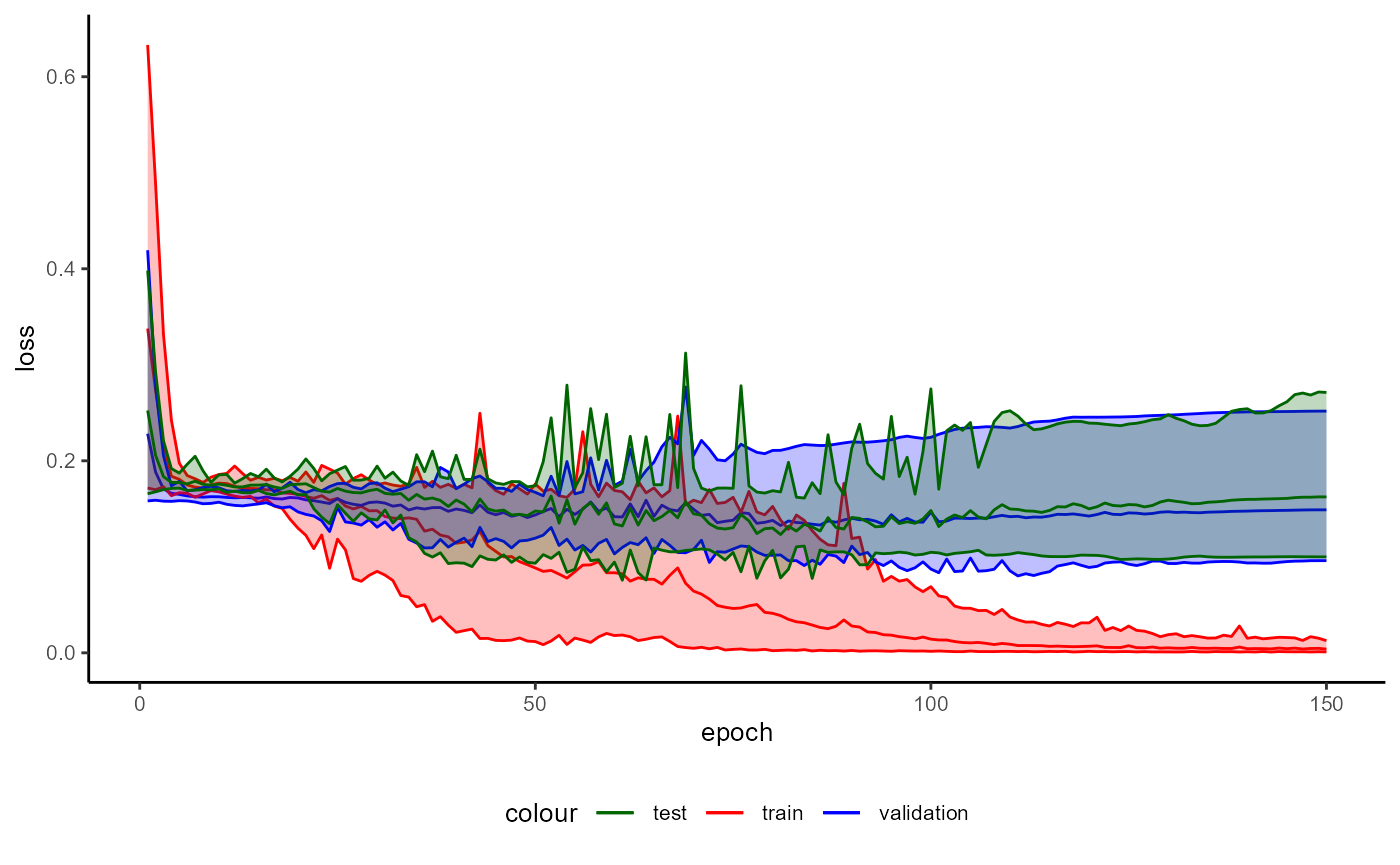
Figure 4: Example of a Training History for a BaseModel.
Sustainability of Training
To explore the ecological impact of the training and fine-tuning of a
model you can call get_sustainability_data("training").
# We use t() to improve the readability of the table
t(base_model_bert$get_sustainability_data("training"))
#>                                      [,1]
#> sustainability_tracked               "TRUE"
#> date                                 "2026-07-06 11:35:30"
#> task                                 "training"
#> sustainability_data.duration_sec     "20.91903"
#> sustainability_data.co2eq_kg         "0.0001921118"
#> sustainability_data.cpu_energy_kwh   "0.0002468855"
#> sustainability_data.gpu_energy_kwh   "0.0001993215"
#> sustainability_data.ram_energy_kwh   "5.808964e-05"
#> sustainability_data.total_energy_kwh "0.0005042967"
#> technical.tracker                    "codecarbon"
#> technical.py_package_version         "3.2.2"
#> technical.cpu_count                  "12"
#> technical.cpu_model                  "12th Gen Intel(R) Core(TM) i5-12400F"
#> technical.gpu_count                  "1"
#> technical.gpu_model                  "1 x NVIDIA GeForce RTX 4070"
#> technical.ram_total_size             "15.84258"
#> region.country_name                  "Germany"
#> region.country_iso_code              "DEU"
#> region.region                        NA
The resulting table provides you detailed information on every single training run with active sustainability tracking.
Sustainability of Inference
Not only the ecological impact of the training is important but also
the energy consumption and CO2-emission during inference. You can
estimate the ecological impact by calling the method
estimate_sustainability_inference_fill_mask.
base_model_bert$estimate_sustainability_inference_fill_mask(
  text_dataset = data_set_reviews_text,
  n = 30,
  sustain_iso_code = "DEU",
  sustain_region = NULL,
  sustain_interval = 15,
  sustain_log_level = "error",
  trace = TRUE
)
#> 2026-07-06 11:35:31 Prepare Data
#> 2026-07-06 11:35:31 Add Masking Token
#> 2026-07-06 11:35:32 Start Sustainability Tracking
#> 2026-07-06 11:35:32 Stop Sustainability Tracking
Here can you provide a text data set which forms the base for
estimating the energy conspumtion during a fill-mask task. With
n you determine the number of texts to be used.
The results of every run can be accessed via
get_sustainability_data("inference").
# We use t() to improve the readability of the table
t(base_model_bert$get_sustainability_data("inference"))
#>                                      [,1]
#> sustainability_tracked               "TRUE"
#> date                                 "2026-07-06 11:35:32"
#> task                                 "FillMask"
#> sustainability_data.duration_sec     "0.5261275"
#> sustainability_data.co2eq_kg         "3.996553e-06"
#> sustainability_data.cpu_energy_kwh   "6.142905e-06"
#> sustainability_data.gpu_energy_kwh   "2.903058e-06"
#> sustainability_data.ram_energy_kwh   "1.445053e-06"
#> sustainability_data.total_energy_kwh "1.049102e-05"
#> technical.tracker                    "codecarbon"
#> technical.py_package_version         "3.2.2"
#> technical.cpu_count                  "12"
#> technical.cpu_model                  "12th Gen Intel(R) Core(TM) i5-12400F"
#> technical.gpu_count                  "1"
#> technical.gpu_model                  "1 x NVIDIA GeForce RTX 4070"
#> technical.ram_total_size             "15.84258"
#> region.country_name                  "Germany"
#> region.country_iso_code              "DEU"
#> region.region                        NA
#> data                                 "empirical data"
#> n                                    "30"
#> batch                                "1"
#> min_seq_len                          NA
#> mean_seq_len                         NA
#> sd_seq_len                           NA
#> max_seq_len                          NA
FLOPS Estimates
Another important value is the total number of FLOPS during training.
These are estimated during every training run. With
get_flops_estimates you receive a table.
# We use t() to improve the readability of the table
t(base_model_bert$get_flops_estimates())
#>               [,1]
#> date          "2026-07-06 11:35:11"
#> approach      "architecture-based"
#> package       "calflops"
#> version       "0.3.2"
#> n_parameter   "184200"
#> batch_size    "12"
#> n_batches     "85"
#> n_epochs      "10"
#> flops_bp_1    "3.124416e+12"
#> flops_bp_2    "4.686624e+12"
#> flops_bp_3    "6.248831e+12"
#> flops_bp_4    "7.811039e+12"
#> flops_counted NA
At the moment only an architecture-based approach is available. The number of FLOPS is not counted directly. Instead it is estimated approximately. The column ‘flops_bp_1’ describes the number of FLOPS for all forwand and backward passes.
Kaplan et al. (2020, p. 7) propose that as a rule of thumb the backward pass has the FLOPS of the forward pass multiplied with factor 2. The resulting FLOPS for all forward and backward passes of a training run are shown in column ‘flops_bp_2’.
All columns do not include computations for a validation or test sample.
3.5 Creating a BaseModel from Hugging Face
In the case you would like to use a pre-trained model from hugging face you can create a base model as follows:
- Chose a model on Hugging Face. Please ensure that the model’s architecture is supported by aifeducation.
- Download the relevant files (model and tokenizer) into a folder on your machine.
- Create an empty base model for the corresponding architecture.
- Call the method
create_from_hfand provide the path the the folder where you stored the model and the tokenizer.
base_model_bert_hf <- BaseModelBert$new()
base_model_bert_hf$create_from_hf(
  model_dir = "examples/bert_uncased",
  tokenizer_dir = "examples/bert_uncased"
)
Now you can use the model as all other base models in aifedcuation. For example, you can train the model as described above or you can use the model as foundation for a TextEmbeddingModel.
4 Text Embedding Models
4.1 Introduction
The text embedding model is used to transform raw texts into
numerical representations. In order to create a new model, you need a
base model that provides the ability to understand natural language. A
text embedding model is stored as an object of class
TextEmbeddingModel.
In aifedcuation, the transformation of raw texts into numbers is a separate step from downstream tasks such as classification. This is to reduce computational time on machines with low performance. By separating text embedding from other tasks, the text embedding has to be calculated only once and can be used for different tasks at the same time. Another advantage is that the training of the downstream tasks involves only the downstream tasks an not the parameters of the embedding model, making training less time-consuming, thus decreasing computational intensity. Finally, this approach allows the analysis of long documents by applying the same algorithm to different parts of a text.
The text embedding model provides a unified interface: After creating the model with different methods, the handling of the model is always the same.
4.2 Create a Text Embedding Model
First you have to choose the base model that forms the foundation of
your new text embedding model. In order to illustrate its use we apply a
pre-trained model from Hugging
Face called EuroBERT-210m.
It is based on the work by Boizard et al. (2025). Download all files
into a new folder. Here we store the model in
"examples/EuroBERT-210m".
We first load the base model as described in section 3.
base_model_eurobert <- BaseModelEuroBert$new()
base_model_eurobert$create_from_hf(
  model_dir = "examples/EuroBERT-210m",
  tokenizer_dir = "examples/EuroBERT-210m"
)
Now we can create the TextEmbeddingModel. At the beginning we have to
chose a value for chunks and for overlap.
Using a transformer model for text embedding is not a problem since your
text does not provide more tokens than the transformer can process. This
maximum value is set in the configuration of the transformer (see
section 3.3). We can request a base model’s maximum sequence length
with:
total_max_seq_len <- base_model_eurobert$get_max_seq_len()
total_max_seq_len
#> [1] 8192
If the text produces more tokens, the last tokens are ignored. In
some instances you might want to analyze long texts. In these
situations, reducing the text to the first tokens (e.g. only the first
512 tokens) could result in a problematic loss of information. To deal
with these situations, you can configure a text embedding model in
aifecuation to split long texts into several chunks which are
processed by the base model. The maximum number of chunks is set with
chunks.
Since transformers are able to account for the context, it may be
useful to interconnect every chunk to bring context into the
calculations. This can be done with overlap to determine
how many tokens of the end of a prior chunk should be added to the
next.
In order to support you in this decision the tokenizer of a BaseModel
can calculate how many chunks are necessary to cover a specific quantile
of texts completely. We illustrate this with an example. Lets assume
that we want an overlap of 128 (token_overlap) tokens
between each chunk. Our BaseModel can process 8192 tokens at maximum. In
this example we use only 512 tokens as the foundation of every text
embedding. Passing these values to the calc_quantiles
method of the tokenizer of our BaseModel reveals the following
quantiles:
chunk_quantile <- base_model_eurobert$Tokenizer$calc_quantiles(
  text_dataset = data_set_reviews_text,
  batch_size = 32L,
  seq_len_tokens = 512L,
  token_overlap = 128L,
  trace = FALSE
)
print(chunk_quantile)
#>     10%     20%     30%     40%     50%     60%     70%     75%     80%     85%
#>       1       1       1       1       1       1       1       1       1       1
#>     90%     95%     99%   99.9%  99.99% 99.999%    100%
#>       2       2       3       3       3       3       3
max_chunks <- chunk_quantile["99.9%"]
If we would like to ensure that about 90% of the texts are completely covered by our text embedding model with the given configuration we need 2 chunks. To ensure that 99.9% of the text are fully represented we need 3 chunks. Here, we choose the 99.9% quantile which requires 3. Altogether, this model can analyse a maximum of 1280 tokens of a text.
Finally, you have to decide from which hidden layer(s) the embeddings
should be drawn. With emb_layer_min and
emb_layer_max you can decide from which layers the average
value for every token should be calculated. Please note that the
calculation considers all layers between emb_layer_min and
emb_layer_max. The maximum number of available layers can
be requested with:
num_layers <- base_model_eurobert$get_n_layers()
num_layers
#> [1] 12
In their initial work, Devlin et al. (2019) used the hidden states of different layers for classification. A study conducted by Liu et al. (2019, p. 1078) investigates the performance of models on 16 linguistic tasks, revealing that for transformers, there is no single best layer, but the best layers are located in an area in the middle and up to the two-thirds layer. Thus, we use the following layers:
eurobert_min_layer <- floor(0.5 * num_layers)
eurobert_min_layer
#> [1] 6

eurobert_max_layer <- ceiling(2 / 3 * num_layers)
eurobert_max_layer
#> [1] 8
With emb_pool_type, you decide which tokens are used for
pooling within every layer. In the case of
emb_pool_type="CLS", only the cls token is used. In the
case of emb_pool_type="Average" all tokens within a layer
are averaged except padding tokens.
With emb_insert_mask_tokens you can request that a
specific percentage of tokens is replaced with the model’s masking
token. This can increase the performance on subsequent tasks. The reason
is that the mask language modeling applied during training does not
match the conditions during application since working with texts outside
training does not require to mask tokens (Meng et al. 2024, p. 1).
The vignette 04 Model configuration and training provides details on how to configure a text embedding model.
Do not forget to pass the base model to the parameter
base_model.
tem <- TextEmbeddingModel$new()
tem$configure(
  model_label = "Text Embedding via EuroBert - 210m",
  model_language = "english",
  max_length = 512,
  chunks = max_chunks,
  overlap = 128,
  emb_layer_min = eurobert_min_layer,
  emb_layer_max = eurobert_max_layer,
  emb_pool_type = "Average",
  base_model = base_model_eurobert,
  emb_insert_mask_tokens = 0.15
)
After deciding about the configuration, you can use your model. You can see the number of learnable parameters of the underlying base model with
tem$BaseModel$count_parameter()
#> [1] 310266624
Another important value is the number of features which you can
request by calling get_n_features.
tem$get_n_features()
#> [1] 768
This number describes the number of dimensions for a text embedding. That is, the number of dimensions which is used to characterize the content of every chunk of text. This value is important as it determines the complexity a classifier or feature extractor has to deal with. Some of classifier’s and feature extractor’s parameters depend on this value. We elaborate this at the relevant point for the different models.
You get a short summary of an object of this class with
print.
print(tem)
#> Object             : TextEmbeddingModel
#> Label              : Text Embedding via EuroBert - 210m
#> Configured         : TRUE
#> BaseModel Type     : BaseModelEuroBert
#> BaseModel Parameter: 310266624
#> Seq. Len.          : 8192
#> Features           : 768
#> N Layer            : 12
#> Vocab Size         : 128000
#> Tokens/Word        :
#> Mask Token         : <|mask|>
#> Pad Token          : <|pad|>
#> Unk token          : NA
#> Chunks             : 3
#> Min Layer          : 6
#> Max Layer          : 8
#> Pooling Type       : Average
4.3 Transforming Raw Texts into Embedded Texts
To transform raw text into a numeric representation, you only have to
use the embed_large method of your model. To do this, you
must provide a LargeDataSetForText to
text_dataset. Relying on the sample data from section 2.3,
we can use the movie reviews as raw texts.
review_embeddings <- tem$embed_large(
  text_dataset = data_set_reviews_text,
  trace = TRUE
)
#> Calculating Embeddings  10.00 % (1|10) done ETA: 0000::00::24Calculating Embeddings  20.00 % (2|10) done ETA: 0000::00::16Calculating Embeddings  30.00 % (3|10) done ETA: 0000::00::13Calculating Embeddings  40.00 % (4|10) done ETA: 0000::00::10Calculating Embeddings  50.00 % (5|10) done ETA: 0000::00::08Calculating Embeddings  60.00 % (6|10) done ETA: 0000::00::06Calculating Embeddings  70.00 % (7|10) done ETA: 0000::00::05Calculating Embeddings  80.00 % (8|10) done ETA: 0000::00::03Calculating Embeddings  90.00 % (9|10) done ETA: 0000::00::02Calculating Embeddings  100.00 % (10|10) done ETA: 0000::00::00
The method embed_largecreates an object of class
LargeDataSetForTextEmbeddings. This is just a data set
consisting of the embeddings of every text. The embeddings are an array,
of which the first dimension refers to specific texts, the second
dimension refers to chunks/sequences, and the third dimension refers to
the features.
You can inspect the data set with print.
print(review_embeddings)
#> Object   : LargeDataSetForTextEmbeddings
#> Columns  : id, input, length
#> Rows     : 300
#> Times    : 3
#> Features : 768
#> Pad Value: -100
With the embedded texts you now have the input to train a new classifier or to apply a pre-trained classifier for predicting categories/classes. In the next chapter we will show you how to use these classifiers. But before we start, we will show you how to save and load your model.
4.4 Saving and Loading Embedded Texts
Since transforming raw texts into text embeddings is time and energy consuming we recommend to save them to disk in order to use the embeddings for further tasks and analysis.
To save the them just call the function save_to_disk as
shown below.
save_to_disk(
  object = review_embeddings,
  dir_path = "examples",
  folder_name = "imdb_movie_reviews"
)
To load the embeddings you can call the function
load_from_disk.
review_embeddings <- load_from_disk("examples/imdb_movie_reviews")4.5 Saving and Loading Text Embedding Models
Saving a created text embedding model is very easy in
aifeducation by using the function save_to_disk.
This function provides a unique interface for all text embedding models.
For saving your work you can pass your model to object and
the directory where to save the model to dir_path. With
folder_name you can determine the name of the folder that
should be created in that directory to store the model.
save_to_disk(
  object = tem,
  dir_path = "examples",
  folder_name = "eurobert_te_model"
)
In this example the model is saved in a folder at the location
examples/robertxml_te_model. If you want to load your model
you can call load_from_disk.
tem <- load_from_disk("examples/eurobert_te_model")4.6 Sustainability
In case the underlying model was trained with an active
sustainability tracker (section 3.2 and 3.3) you can receive a table
showing you the energy consumption, CO2 emissions, and hardware used
during training by calling
BaseModel$get_sustainability_data("training"). For our
example this would be
tem$BaseModel$get_sustainability_data("training").
4.7 Training History
If you would like to see the training history of the underlying base model you can call a special method.
tem$BaseModel$plot_training_history(
  ind_best_model = TRUE
)
Please note that this plot is not available for this example since the necessary data is not directly available for this model on Hugging Face. If you train a model with this package the training history is always saved.
5 Overview Classifiers
Classifiers are built on top of a TextEmbeddingModel.
They use the embedded texts produced by these models and predict
classes/categories. You can build your classifier with the help of two
components.
First, you choose a core model. It determines where different layers are located and how the outputs of the different layers are combined into the final output of the model.
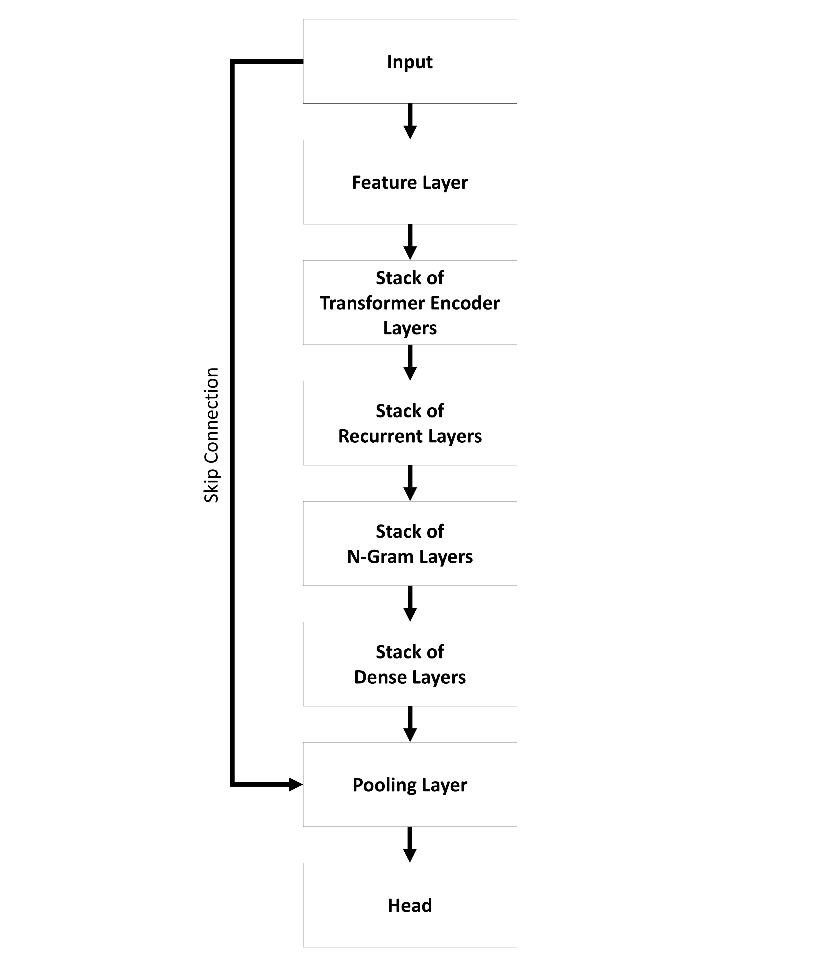
The sequential architecture (Figure 5) provides models where the input is passed to a specific number of layers step by step. All layers are grouped by their kind into stacks.
In contrast, the parallel architecture (Figure 6) offers a model where an input is passed to different types of layers separately. At the end the outputs are combined to create the final output of the whole model.
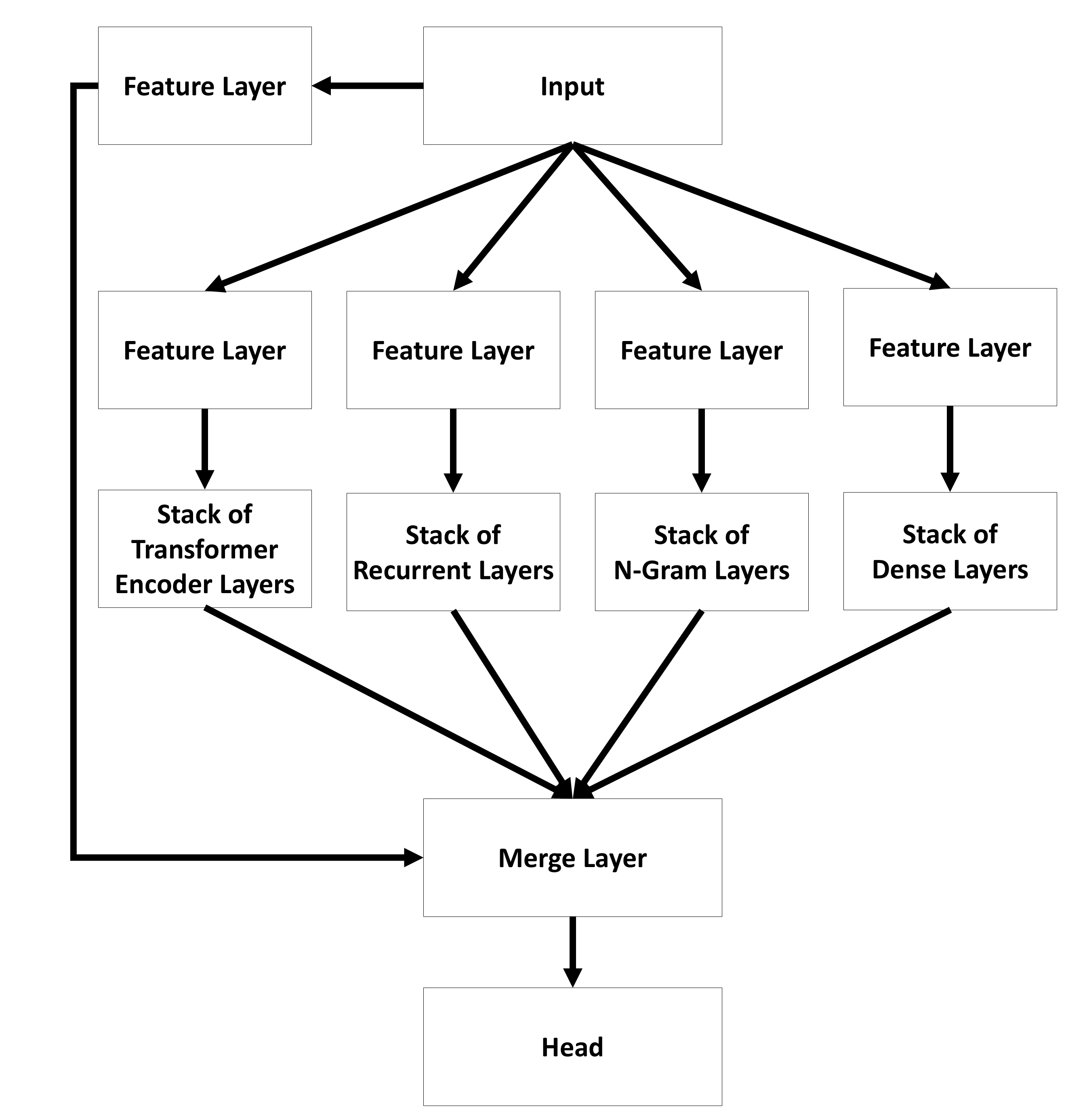
You can find the name of the used core model in the name of the
classifiers. For example TEClassifierSequential uses a
sequential core model while TEClassifierParallel
uses a parallel core model.
In general, all layers within a core model allow further customization allowing you to build a high number of different models.
A detailed description of all layers can be found in vignette A01 Layers and Stack of Layers:
Second, you can choose how the core model is used for classification. At the moment a probability and metric based classifier is possible.
- Probability Based Classifiers: Probability classifiers are used to predict a probability distribution for different classes/categories. This is the standard case most common in literature.
- Prototype Based Classifiers: Prototype based classifiers are a kind of metric based classifiers. Here the classifiers do not predict a probability distribution. Instead it calculates a prototype for every class/category and measures the distance between a case and all prototypes. The class/category of the prototype with the smallest distance to the case is assigned to that case. In contrast to the probability classifiers these models can handle classes/categories that were not part of the training. For more details please refer to section 7.
The training of a classifier consists of two stages. The first stage aims to estimate the performance of the model while the second stage trains the model for application.
For performance estimation, training splits the data into several
chunks based on cross-fold validation. The number of folds is set with
data_folds. In every case, one fold is not used for
training and serves as a test sample. The remaining data is
used to create a training and a validation sample. The
percentage of cases within each fold used as a validation sample is
determined with data_val_size. This sample is used to
determine the state of the model that generalizes best. All performance
values saved in the trained classifier refer to the test sample. This
data has never been used during training and provides a more realistic
estimation of a classifier’s performance.
Since aifedcuation tries to address the special needs in educational and social science, some special training steps are integrated for all models.
Synthetic Cases: In case of imbalanced data, it is recommended to augment your data. Before training, a number of new units is created via different techniques. Currently you can request the K-Nearest Neighbor OveRsampling Approach (KNNOR) developed by Islam et al. (2022). The aim is to create new cases that fill the gap to the majority class. Multi-class problems are reduced to a two class problem (class under investigation vs. all others) for generating these units. If the technique allows to set the number of neighbors during generation, you can configure the data generation with
sc_min_kandsc_max_k. The synthetic cases for every class are generated for all k betweensc_min_kandsc_max_k. Every k contributes proportionally to the synthetic cases.Pseudo-Labeling: This technique is relevant if you have labeled target data and a large number of unlabeled target data. The idea is to integrate the unlabeled into training to increase performance and to avoid high costs by labeling a high number of cases manually. With the different parameters starting with
pl_, you can configure the process of pseudo-labeling. Implementation of pseudo-labeling is based on Cascante-Bonilla et al. (2020). To apply pseudo-labeling, you have to setuse_pl=TRUE.pl_max=1.00,pl_anchor=1.00, andpl_min=0.00are used to describe the certainty of a prediction. 0 refers to random guessing while 1 refers to perfect certainty.pl_anchoris used as a reference value. The distance topl_anchoris calculated for every case. Then, they are sorted with an increasing distance frompl_anchor. The proportion of added pseudo-labeled data into training increases with every step. The maximum number of steps is determined withpl_max_steps. Cases close topl_anchorare included first.
Figure 7 illustrates the training loop for the cases that all options
are set to TRUE.
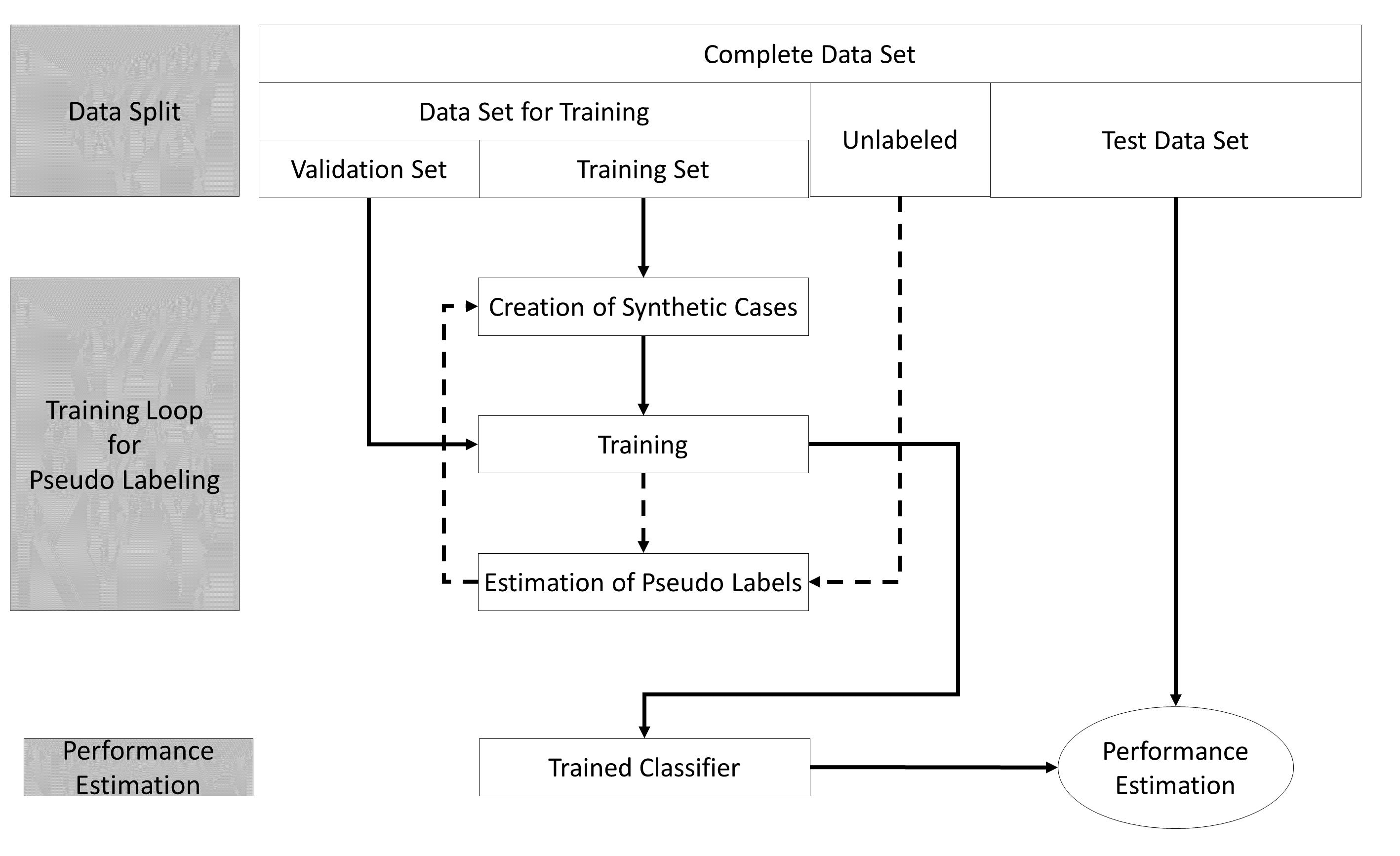
The example stated in the Figure applies the generation of synthetic
cases and the algorithm proposed by Cascante-Bonilla et al. (2020). For
every fold, the training starts with generating synthetic cases to fill
the gap between the classes and the majority class. After this, an
initial training of the classifiers starts. The trained classifier is
used to predict pseudo-labels for the unlabeled part of the data and
adds 20% of the cases with the highest certainty for their pseudo-labels
to the training data set. Now new synthetic cases are generated based on
both the labeled data and the newly added pseudo-labeled data. The
classifier is re-initialized and trained again. After training, the
classifier predicts the potential labels of all originally
unlabeled data and adds 40% of the pseudo-labeled data to the training
data with the highest certainty. Again, new synthetic cases are
generated on both the labeled and added pseudo-labeled data. The model
is again re-initialized and trained again until the maximum number of
steps for pseudo labeling (pl_max_steps) is reached. After
this, the logarithm is restated for the next fold until the number of
folds (data_folds) is reached. All of these steps are only
used to estimate the performance of the classifier to evaluate for
unknown data.
The last phase of the training begins after the last fold. In the final training, the data set is split only into a training and validation set without a test set to provide the maximum amount of data for the best performance in final training. All configurations of the performance estimation phase are used in the final training phase.
Please note that creating, training, and predicting works for all types of classifiers as described in the chapters below.
6 Probability Based Classifiers
6.1 Creation
To show you how to create a classifier we use a classifier of class
TEClassifierSequential as an example. With the sample data
from section 2.3 and the text embeddings from section 4.3, the creation
of a new classifier may look like:
classifier <- TEClassifierSequential$new()
classifier$configure(
  label = "Classifier for Estimating a Postive or Negative Rating of Movie Reviews",
  text_embeddings = review_embeddings,
  feature_extractor = NULL,
  target_levels = c("neg", "pos"),
  skip_connection_type = "ResidualGate",
  cls_pooling_features = 20,
  cls_pooling_type = "MaxTimes",
  cls_head_type = "Regular",
  feat_act_fct = "Tanh",
  feat_size = 384,
  feat_bias = TRUE,
  feat_dropout = 0.0,
  feat_parametrizations = "None",
  feat_normalization_type = "PowerNorm",
  ng_conv_act_fct = "GELU",
  ng_conv_n_layers = 1,
  ng_conv_ks_min = 2,
  ng_conv_ks_max = max_chunks,
  ng_conv_bias = FALSE,
  ng_conv_dropout = 0.05,
  ng_conv_parametrizations = "None",
  ng_conv_normalization_type = "PowerNorm",
  ng_conv_residual_type = "ResidualGate",
  dense_act_fct = "GELU",
  dense_n_layers = 2,
  dense_dropout = 0.30,
  dense_bias = FALSE,
  dense_parametrizations = "None",
  dense_normalization_type = "PowerNorm",
  dense_residual_type = "ResidualGate",
  rec_act_fct = "Tanh",
  rec_n_layers = 0,
  rec_type = "GRU",
  rec_bidirectional = FALSE,
  rec_dropout = 0.2,
  rec_bias = FALSE,
  rec_parametrizations = "None",
  rec_normalization_type = "PowerNorm",
  rec_residual_type = "ResidualGate",
  tf_act_fct = "SwiGLU",
  tf_dense_dim = ceiling(2.67 * 64),
  tf_n_layers = 0,
  tf_dropout_rate_1 = 0.1,
  tf_dropout_rate_2 = 0.3,
  tf_attention_type = "MultiHead",
  tf_positional_type = "absolute",
  tf_num_heads = 12,
  tf_bias = FALSE,
  tf_parametrizations = "None",
  tf_normalization_type = "PowerNorm",
  tf_normalization_position = "Pre",
  tf_residual_type = "ResidualGate"
)
Similarly to the text embedding model, you should provide a label
(label) for your new classifier. With
text_embeddings you have to provide a
LargeDataSetForTextEmbeddings. The data set is created with
a TextEmbeddingModel as described in section 4. We here
continue our example and use the embeddings produced by our BERT
model.
target_levels take the categories/classes you classifier
should predict. This can be numbers or even words.
In case you would like to use ordinal data, it is very important that you provide the classes/categories in the correct order. That is, classes/categories representing a “higher” level must be stated after categories/classes with a “lower” level. If you provide the wrong order, the performance indices are not valid. In case of nominal data the order does not matter.
With feature_extractor you can add a feature extractor
that tries to reduce the number of features of your text embeddings
before passing the embeddings to the classifier. You can read more on
this in section 8.
With the help of the other parameters you can define the complexity and abilities of your model. A description of the different models can be found in A01 Layers and Stack of Layers.
Please note that you have to choose the parameter
feat_size depending on the number of features of the
underlying text embedding model. You can request this number by calling
the method get_n_features of the used text embedding model.
In our example this would be:
tem$get_n_features()
#> [1] 768
The number for feat_size should be equal to or less than
this value, since this layer tries to compress the text embeddings into
fewer dimensions. While this reduces the number of of parameters for all
subsequent layers and decreases training and usage time, it may result
in information loss. You can experiment with this value to strike a
balance between speed and performance. A study by Takeshita et
al. (2025) shows that randomly dropping 50% of the dimensions leads only
to a minor drop in performance in classification tasks. Thus, this value
can serve as a rule of thumb for determining this parameter.
In our example we have only a very limited number of samples. Thus, we decrease the number of features further.
In addition, the parameter cls_pooling_features should
be equal or less the number you used for feat_size. With
cls_pooling_features you determine how many of the
resulting features should be used for classification. Thus, this value
acts as a filter.
The vignette 04 Model configuration and training provides details on how to configure a classifier.
In our example we use only two n-gram layers
(ng_conv_n_layers = 1) and two dense layers
(dense_n_layers = 2). All other layers are omitted from the
model by setting the number of layers to zero
(tf_n_layers = 0,rec_n_layers = 0).
As pooling method we use minimum and maximum over time
(cls_pooling_type="MinMaxTimes"). That is, the highest and
the lowest features within every feature dimension are used for
calculating the classes/labels. The cls_pooling_features is
only relevant if you set cls_pooling_type to
"Min", "Max" or "MinMax". These
three options request an additional pooling over features which in most
times leads to a lose of information. They are useful only if your
classifier has to predict two classes/categories.
In this example we use a regular classification head
(cls_head_type = "Regular") where all neurons of the
previous layer are connected all classes. Li et al. (2020)[https://doi.org/10.1109/TIP.2020.2990277] proposed a
special classification head
(cls_head_type = "PairwiseOrthogonal"). This layer allows
every neuron only to establish a connection to a single class. For this
special layer you can add a dense layer before the classification head
(cls_head_type = "PairwiseOrthogonalDense") in order to
improve performance with high rates for dropout in the previous
layers.
You receive a short summary of the classifier by calling
print.
print(classifier)
#> Object    : TEClassifierSequential
#> ID        : cls_amcb41R0ZLBKZwh2
#> Label     : Classifier for Estimating a Postive or Negative Rating of Movie Reviews
#> Configured: TRUE
#> Trained   : FALSE
#> Classes   : neg, pos
#> Times     : 3
#> Features  : 768
#> Parameter : 962696
#> req. FE   : FALSE
After you have created a new classifier, you can begin training. You can see the number of learnable parameters of your model with:
classifier$count_parameter()
#> [1] 962696
6.2 Training
To start the training of your classifier, you have to call the
train method. Similarly, for the creation of the
classifier, you must provide the text embeddings to
data_embeddings and the categories/classes as target data
to data_targets. Please remember that
data_targets expects a named factor where
the names correspond to the IDs of the corresponding text embeddings.
Text embeddings and target data that cannot be matched are omitted from
training.
classifier$train(
  data_embeddings = review_embeddings,
  data_targets = review_labels,
  data_folds = 10,
  data_val_size = 0.25,
  loss_balance_class_weights = TRUE,
  loss_balance_sequence_length = TRUE,
  loss_cls_fct_name = "FocalLoss",
  use_sc = TRUE,
  sc_method = "knnor",
  sc_min_k = 1,
  sc_max_k = 10,
  use_pl = FALSE,
  pl_max_steps = 3,
  pl_max = 1.00,
  pl_anchor = 1.00,
  pl_min = 0.00,
  sustain_track = TRUE,
  sustain_iso_code = "DEU",
  sustain_region = NULL,
  sustain_interval = 15,
  sustain_log_level = "error",
  epochs = 2000,
  batch_size = 32,
  trace = TRUE,
  ml_trace = 0,
  log_dir = NULL,
  log_write_interval = 10,
  n_cores = auto_n_cores(),
  lr_rate = 0.0,
  lr_min = 0.0,
  lr_scheduler = "None",
  lr_warm_up_ratio = 0.05,
  optimizer = "AdamW",
  amp = TRUE
)
#> 2026-07-06 11:35:55 Total Cases: 300 Unique Cases: 300 Labeled Cases: 225
#> 2026-07-06 11:35:58 Start
#> 2026-07-06 11:35:58 Start Sustainability Tracking
#> 2026-07-06 11:35:58 Estimating Learning Rates
#> integer(0)
#> 2026-07-06 11:36:45 Set lr_rate to 5e-05 and lr_min to 5e-06.
#> 2026-07-06 11:36:45 | Iteration 1 from 10
#> 2026-07-06 11:36:45 | Iteration 1 from 10 | Generating synthetic cases
#> 2026-07-06 11:36:53 | Iteration 1 from 10 | Generating synthetic cases done
#> 2026-07-06 11:36:53 | Iteration 1 from 10 | Training
#> integer(0)
#> Data Set Type: Test | ELC: 1647 | Loss 0.0046 | ACC: 0.9091 | BACC: 0.8571 | Avg. Iota: 0.7983 | Smoothed Avg. Iota: 0.7294
#> 2026-07-06 11:41:22 | Iteration 2 from 10
#> 2026-07-06 11:41:22 | Iteration 2 from 10 | Generating synthetic cases
#> 2026-07-06 11:41:44 | Iteration 2 from 10 | Generating synthetic cases done
#> 2026-07-06 11:41:44 | Iteration 2 from 10 | Training
#> integer(0)
#> Data Set Type: Test | ELC: 917 | Loss 0.0130 | ACC: 0.9091 | BACC: 0.8952 | Avg. Iota: 0.8125 | Smoothed Avg. Iota: 0.7632
#> 2026-07-06 11:43:38 | Iteration 3 from 10
#> 2026-07-06 11:43:38 | Iteration 3 from 10 | Generating synthetic cases
#> 2026-07-06 11:43:47 | Iteration 3 from 10 | Generating synthetic cases done
#> 2026-07-06 11:43:47 | Iteration 3 from 10 | Training
#> integer(0)
#> Data Set Type: Test | ELC: 1491 | Loss 0.0267 | ACC: 0.7727 | BACC: 0.6810 | Avg. Iota: 0.5559 | Smoothed Avg. Iota: 0.5652
#> 2026-07-06 11:48:13 | Iteration 4 from 10
#> 2026-07-06 11:48:13 | Iteration 4 from 10 | Generating synthetic cases
#> 2026-07-06 11:48:37 | Iteration 4 from 10 | Generating synthetic cases done
#> 2026-07-06 11:48:37 | Iteration 4 from 10 | Training
#> integer(0)
#> Data Set Type: Test | ELC: 1026 | Loss 0.0264 | ACC: 0.8182 | BACC: 0.8286 | Avg. Iota: 0.6750 | Smoothed Avg. Iota: 0.6283
#> 2026-07-06 11:51:21 | Iteration 5 from 10
#> 2026-07-06 11:51:21 | Iteration 5 from 10 | Generating synthetic cases
#> 2026-07-06 11:51:30 | Iteration 5 from 10 | Generating synthetic cases done
#> 2026-07-06 11:51:30 | Iteration 5 from 10 | Training
#> integer(0)
#> Data Set Type: Test | ELC: 1926 | Loss 0.0016 | ACC: 0.9545 | BACC: 0.9667 | Avg. Iota: 0.9042 | Smoothed Avg. Iota: 0.7463
#> 2026-07-06 11:56:17 | Iteration 6 from 10
#> 2026-07-06 11:56:17 | Iteration 6 from 10 | Generating synthetic cases
#> 2026-07-06 11:56:28 | Iteration 6 from 10 | Generating synthetic cases done
#> 2026-07-06 11:56:28 | Iteration 6 from 10 | Training
#> integer(0)
#> Data Set Type: Test | ELC: 4 | Loss 0.0075 | ACC: 0.4783 | BACC: 0.6000 | Avg. Iota: 0.3000 | Smoothed Avg. Iota: 0.3258
#> 2026-07-06 12:00:52 | Iteration 7 from 10
#> 2026-07-06 12:00:52 | Iteration 7 from 10 | Generating synthetic cases
#> 2026-07-06 12:01:11 | Iteration 7 from 10 | Generating synthetic cases done
#> 2026-07-06 12:01:11 | Iteration 7 from 10 | Training
#> integer(0)
#> Data Set Type: Test | ELC: 1855 | Loss 0.0068 | ACC: 0.7391 | BACC: 0.7125 | Avg. Iota: 0.5606 | Smoothed Avg. Iota: 0.4581
#> 2026-07-06 12:05:46 | Iteration 8 from 10
#> 2026-07-06 12:05:46 | Iteration 8 from 10 | Generating synthetic cases
#> 2026-07-06 12:06:10 | Iteration 8 from 10 | Generating synthetic cases done
#> 2026-07-06 12:06:10 | Iteration 8 from 10 | Training
#> integer(0)
#> Data Set Type: Test | ELC: 1062 | Loss 0.0347 | ACC: 0.8261 | BACC: 0.7792 | Avg. Iota: 0.6667 | Smoothed Avg. Iota: 0.6528
#> 2026-07-06 12:08:40 | Iteration 9 from 10
#> 2026-07-06 12:08:40 | Iteration 9 from 10 | Generating synthetic cases
#> 2026-07-06 12:08:48 | Iteration 9 from 10 | Generating synthetic cases done
#> 2026-07-06 12:08:48 | Iteration 9 from 10 | Training
#> integer(0)
#> Data Set Type: Test | ELC: 630 | Loss 0.0125 | ACC: 0.8696 | BACC: 0.8708 | Avg. Iota: 0.7563 | Smoothed Avg. Iota: 0.6309
#> 2026-07-06 12:10:54 | Iteration 10 from 10
#> 2026-07-06 12:10:54 | Iteration 10 from 10 | Generating synthetic cases
#> 2026-07-06 12:11:17 | Iteration 10 from 10 | Generating synthetic cases done
#> 2026-07-06 12:11:17 | Iteration 10 from 10 | Training
#> integer(0)
#> Data Set Type: Test | ELC: 1134 | Loss 0.0167 | ACC: 0.8261 | BACC: 0.7792 | Avg. Iota: 0.6667 | Smoothed Avg. Iota: 0.6704
#> 2026-07-06 12:14:11 | Final training
#> 2026-07-06 12:14:11 | Final training | Generating synthetic cases
#> 2026-07-06 12:14:40 | Final training | Generating synthetic cases done
#> 2026-07-06 12:14:40 | Final training | Training
#> integer(0)
#> Data Set Type: Validation | ELC: 1053 | Loss 0.0100 | ACC: 0.8000 | BACC: 0.7658 | Avg. Iota: 0.6330 | Smoothed Avg. Iota: 0.6155
#> 2026-07-06 12:17:20 Stop Sustainability Tracking
#> 2026-07-06 12:17:20 Training Complete
You can further modify the training process with different arguments.
With loss_balance_class_weights=TRUE the absolute
frequencies of the classes/categories are adjusted according to the
‘Inverse Class Frequency’ method. This option should be activated if you
have to deal with imbalanced data.
With loss_balance_sequence_length=TRUE you can increase
performance if you have to deal with texts that differ in their lengths
and have an imbalanced frequency. If this option is enabled, the loss is
adjusted to the absolute frequencies of length of your texts according
to the ‘Inverse Class Frequency’ method.
epochs determines the maximal number of epochs. During
training, the model with the best balanced accuracy is saved and
used.
batch_size sets the number of cases to be processed
simultaneously. It is a very important parameter with a significant
impact on the model’s performance due to the generalisation gap (Keskar
et al., 2017 p. 2). The generalisation gap describes the observation
that large batch sizes tend to poor generalisation performance on test
datasets compared to models trained with a small batch size (Keskar et
al., 2017 p. 3). A study conducted by Masters and Luschi (2018) suggests
ways to achieve good batch size for using "SGD" as
optimizer. Their study shows that smaller batch sizes offer more stable
and reliable training and at the same time achieve better generalisation
performance. Batch sizes between 4 and 32 lead to the best
performance.
We set lr_rate = 0.0 and lr_min = 0.0 to
request an automatic calculation for a good learning rate.
To speed up computations we activate automatic mixed precision (amp)
with gradient scaling by setting amp = TRUE. In general we
recommend to activate mixed precision. If you encounter any problems
turn this option off.
Please note that there are exceptions to this rule. In the context of contrastive learning, higher batch sizes tend to generate better generalisation performance (Chen et al., 2020). For more details please refer to the vignette 04 Model configuration and training
Since training a neural net is energy consuming,
aifeducation allows you to estimate its ecological impact with
the help of the python library codecarbon. Thus,
sustain_track is set to TRUE by default. If
you use the sustainability tracker you must provide the alpha-3 code for
the country where your computer is located (e.g., “CAN”=“Canada”,
“DEU”=“Germany”). A list with the codes can be found on Wikipedia.
The reason is that different countries use different sources and
techniques for generating their energy resulting in a specific impact on
CO2 emissions. For the USA and Canada, you can additionally specify a
region by setting sustain_region. Please refer to the
documentation of ‘codecarbon’ for more information.
Finally, trace and ml_trace allow you to
control how much information about the training progress is printed to
the console.
Please note that training the classifier can take some time. In case
options like the generation of synthetic cases (use_sc) or
pseudo-labeling (use_pl) are disabled, the training process
is shorter.
Please note that after performance estimation, the final training of the classifier makes use of all data available. That is, the test sample is left empty.
In order to visualize the progress of training you can request a plot
which shows how important performance measures develop over epochs. You
can choose between classifier’s loss ("loss"), accuracy
("accuracy"),
balanced accuracy ("balanced_accuracy"), and average
iota("avg_iota"). Set final_training=FALSE to
request mean values of all folds used during the performance estimation
phase.
classifier$plot_training_history(
  final_training = FALSE,
  pl_step = NULL,
  measure = "loss",
  ind_best_model = FALSE,
  ind_selected_model = TRUE,
  x_min = NULL,
  x_max = NULL,
  y_min = NULL,
  y_max = NULL,
  add_min_max = FALSE,
  text_size = 10
)
Figure 8: Training History of a Classifier during Performance Estimation Stage (loss)
Figure 8 shows the development of the loss as a mean of all folds. In general the curve for training should decrease to zero. The curves for the validation and test sample should decrease and start increasing after a certain point. The rectangles indicate the state of the model that was selected as the best state during a fold.
Since the there are some measures which provide a better interpretation as the loss you can request further plots. The following plot shows the development of average iota for all categories/classes.
classifier$plot_training_history(
  final_training = FALSE,
  pl_step = NULL,
  measure = "avg_iota",
  ind_best_model = FALSE,
  ind_selected_model = TRUE,
  x_min = NULL,
  x_max = NULL,
  y_min = NULL,
  y_max = 1L,
  add_min_max = FALSE,
  text_size = 10
)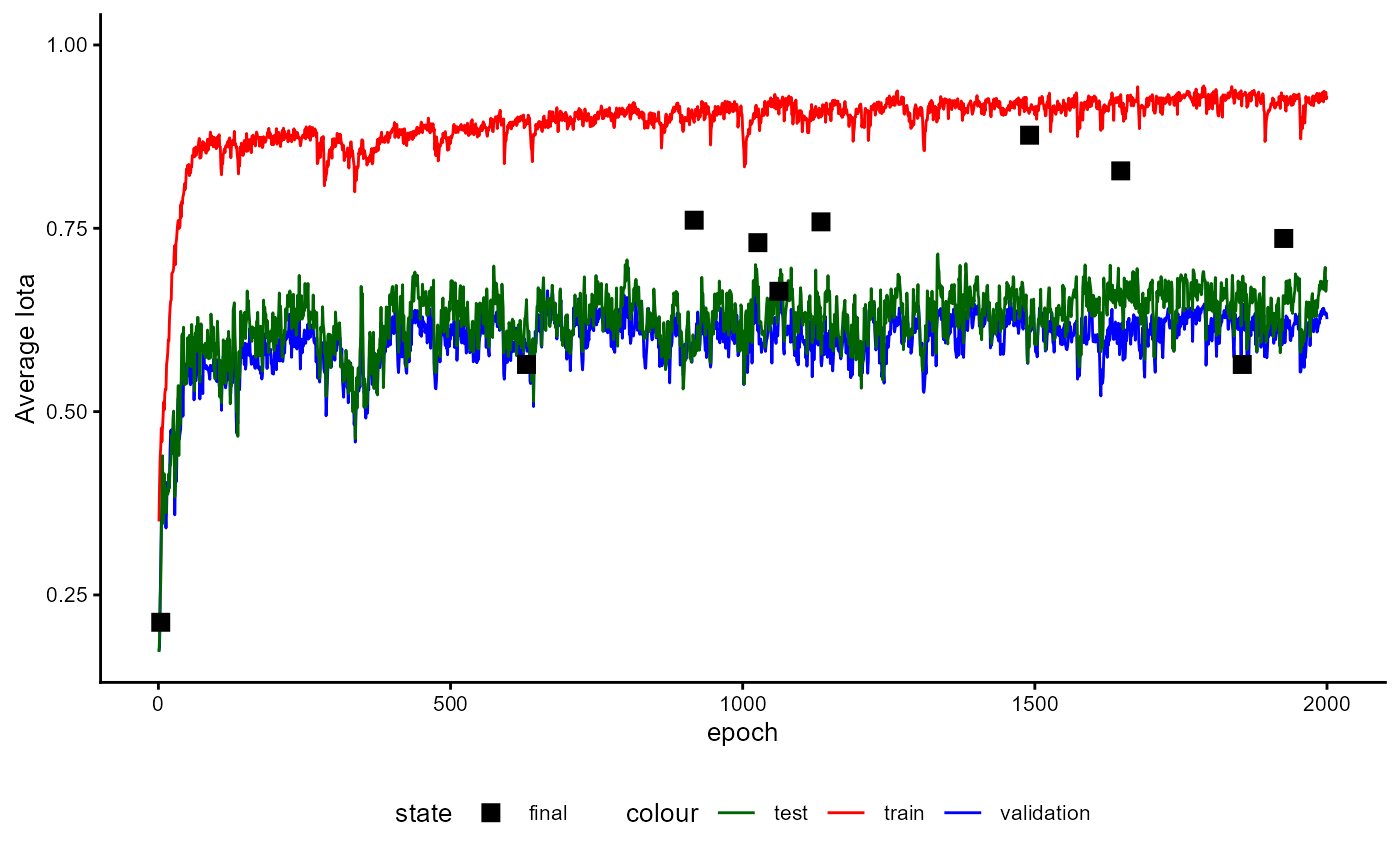
Figure 9: Training History of a Classifier during Performance Estimation Stage (iota)
Average iota ranges between 0and 1 and
indicates how good the predictions represent the true values. Higher
values indicate a better performance.
Since measures such as average iota are measures for discrete values that can heavily fluctuate you can plot a smoothed version of average iota which is more precise.
classifier$plot_training_history(
  final_training = FALSE,
  pl_step = NULL,
  measure = "s_avg_iota",
  ind_best_model = FALSE,
  ind_selected_model = TRUE,
  x_min = NULL,
  x_max = NULL,
  y_min = NULL,
  y_max = 1L,
  add_min_max = FALSE,
  text_size = 10
)
Figure 10: Training History of a Classifier during Performance Estimation Stage (smoothed iota)
To see the training process of the final training stage you have to
set final_training=TRUE as shown in the following
Figures.
classifier$plot_training_history(
  final_training = TRUE,
  pl_step = NULL,
  measure = "loss",
  ind_best_model = FALSE,
  ind_selected_model = TRUE,
  x_min = NULL,
  x_max = NULL,
  y_min = NULL,
  y_max = NULL,
  add_min_max = FALSE,
  text_size = 10
)
Figure 11: Training History of a Classifier during Final Training Stage (loss)
The dotted line indicates the final model state. Please note that in many times this state is not the state with the lowest value on the validation loss because the best model is selected by applying several criteria in a hierarchical order. The first criterion is model’s performance on average iota, the second it`s performance on balanced accuracy, and the third critertion is the loss.
classifier$plot_training_history(
  final_training = TRUE,
  pl_step = NULL,
  measure = "avg_iota",
  ind_best_model = FALSE,
  ind_selected_model = TRUE,
  x_min = NULL,
  x_max = NULL,
  y_min = NULL,
  y_max = 1L,
  add_min_max = FALSE,
  text_size = 10
)
Figure 12: Training History of a Classifier during Final Training Stage (iota)
classifier$plot_training_history(
  final_training = TRUE,
  pl_step = NULL,
  measure = "s_avg_iota",
  ind_best_model = FALSE,
  ind_selected_model = TRUE,
  x_min = NULL,
  x_max = NULL,
  y_min = NULL,
  y_max = 1L,
  add_min_max = FALSE,
  text_size = 10
)
Figure 13: Training History of a Classifier during Final Training Stage (smoothed iota)
In order to have a deeper insight into training you can request a
plot that visualizes the calculation of the learning rate. Please note
that this plot is only available if you have set
lr_rate = 0.0 or lr_min = 0.0.
classifier$plot_learning_rate()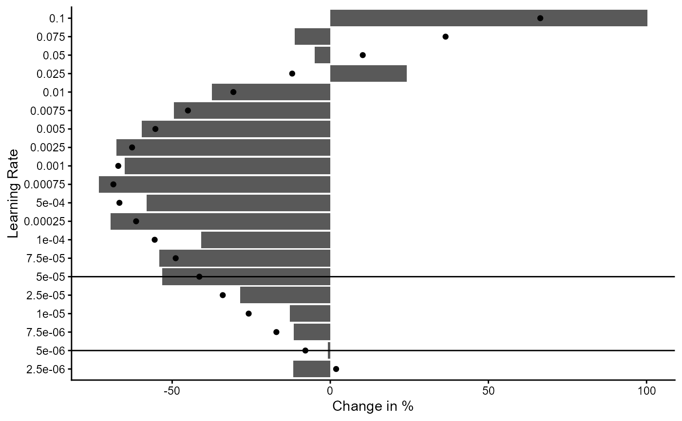
Figure 14: Analysis of Different Learning Rates
The bars of the plot shows how much the loss increases or decreases compared to the initial loss. The values express the degree in percentage to the initial loss. A decrease is desired.The points of the plot show a smoothed distribution of the loss. All calculations for selecting a good maximum and minimum learning rate are based on the smoothed data. The automatic calculation selects the learning rate from the longest range of learning rates that lead to a decreased loss. The maximum learning rate is set as the learning rate where the decrease in the loss has a turning point. The minimum is set to the learning rate that has the smallest reduction of the loss.
6.3 Performance Evaluation
After finishing training, you can evaluate the performance of the classifier. For every fold, the classifier is applied to the test sample and the results are compared to the true categories/classes. Since the test sample is never part of the training, all performance measures provide a more realistic idea of the classifier’s performance.
To support researchers in judging the quality of the predictions, aifeducation utilizes several measures and concepts from content analysis. These are
- Iota Concept of the Second Generation (Berding & Pargmann 2022).
- Krippendorff’s Alpha (Krippendorff 2019).
- Percentage Agreement.
- Gwet’s AC1/AC2 (Gwet 2014).
- Kendall’s coefficient of concordance W.
- Cohen’s Kappa unweighted (Cohen 1960).
- Cohen’s Kappa with equal weights (Cohen 1968).
- Cohen’s Kappa with squared weights (Cohen 1968).
- Fleiss’ Kappa for multiple raters without exact estimation (Fleiss 1971).
You can access the concrete values as mean values across all folds
via reliability$test_metric_mean. In our example this would
be:
classifier$reliability$test_metric_mean
#>           iota_index            min_iota2            avg_iota2
#>            0.6642292            0.5779942            0.6696096
#>            max_iota2            min_alpha            avg_alpha
#>            0.7612251            0.6675000            0.7970238
#>            max_alpha    static_iota_index   dynamic_iota_index
#>            0.9265476            0.3889690            0.5716826
#>       kalpha_nominal       kalpha_ordinal              kendall
#>            0.5784880            0.5784880            0.8078313
#>   c_kappa_unweighted       c_kappa_linear      c_kappa_squared
#>            0.5961613            0.5961613            0.5961613
#>         kappa_fleiss percentage_agreement    balanced_accuracy
#>            0.5689657            0.8102767            0.7970238
#>     gwet_ac1_nominal      gwet_ac2_linear   gwet_ac2_quadratic
#>            0.6582657            0.6582657            0.6582657
#>        avg_precision           avg_recall               avg_f1
#>            0.8255213            0.7970238            0.7844828
An addition, standard measures from machine learning are reported. These are
- Precision
- Recall
- F1-Score
You can access these values as follows:
classifier$reliability$standard_measures_mean
#>     precision    recall        f1
#> neg 0.7618254 0.7607143 0.7367793
#> pos 0.8892171 0.8333333 0.8321863
Finally, you can plot a coding stream scheme showing how the cases of different classes are labeled.
classifier$plot_coding_stream()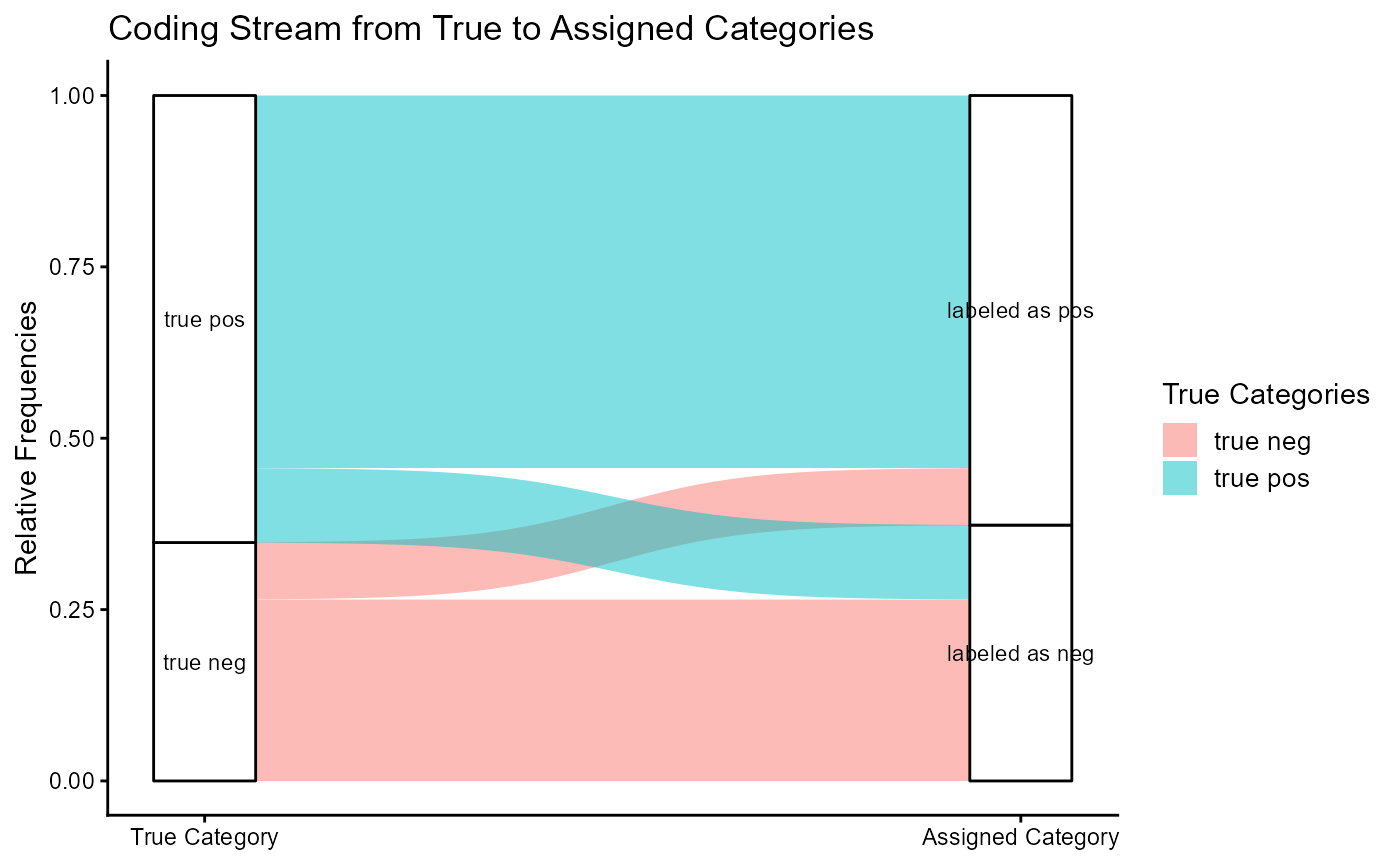
Figure 15: Coding Stream of the Classifier
Evaluating the performance of a classifier is a complex task and and beyond the scope of this vignette. Instead, we would like to refer to the cited literature of content analysis and machine learning if you would like to dive deeper into this topic.
6.4 Sustainability
In case the classifier was trained with an active sustainability
tracker, you can receive information on sustainability by calling
classifier$get_sustainability_data().
# We use t() to improve the readability of the table
t(classifier$get_sustainability_data())
#>                                      [,1]
#> sustainability_tracked               "TRUE"
#> date                                 "2026-07-06 12:17:20"
#> task                                 NA
#> sustainability_data.duration_sec     "2482.383"
#> sustainability_data.co2eq_kg         "0.02020169"
#> sustainability_data.cpu_energy_kwh   "0.0293018"
#> sustainability_data.gpu_energy_kwh   "0.01683348"
#> sustainability_data.ram_energy_kwh   "0.006894486"
#> sustainability_data.total_energy_kwh "0.05302977"
#> technical.tracker                    "codecarbon"
#> technical.py_package_version         "3.2.2"
#> technical.cpu_count                  "12"
#> technical.cpu_model                  "12th Gen Intel(R) Core(TM) i5-12400F"
#> technical.gpu_count                  "1"
#> technical.gpu_model                  "1 x NVIDIA GeForce RTX 4070"
#> technical.ram_total_size             "15.84258"
#> region.country_name                  "Germany"
#> region.country_iso_code              "DEU"
#> region.region                        NA
6.5 Saving and Loading a Classifier
Saving and loading follows the same pattern as for the other objects
in aifeducation. You can save the classifier by calling
save_to_disk. In our example this may be:
save_to_disk(
  object = classifier,
  dir_path = "examples",
  folder_name = "cls_imdb_movie_reviews"
)
The classifier is saved to
examples/cls_imdb_movie_reviews. To load the model call
load_from_disk.
classifier <- load_from_disk("examples/cls_imdb_movie_reviews")6.6 Predicting New Data
If you would like to apply your classifier to new data, two steps are necessary. You must first transform the raw text into a numerical representation by using exactly the same text embedding model that was used to train your classifier (see section 4). In the case of our example classifier, we use our BERT model.
# If our model is not loaded
tem <- load_from_disk("examples/eurobert_te_model")

# Create a numerical representation of the text
review_embeddings <- tem$embed_large(
  text_dataset = data_set_reviews_text,
  trace = TRUE
)
#> Calculating Embeddings  10.00 % (1|10) done ETA: 0000::00::18Calculating Embeddings  20.00 % (2|10) done ETA: 0000::00::13Calculating Embeddings  30.00 % (3|10) done ETA: 0000::00::11Calculating Embeddings  40.00 % (4|10) done ETA: 0000::00::09Calculating Embeddings  50.00 % (5|10) done ETA: 0000::00::07Calculating Embeddings  60.00 % (6|10) done ETA: 0000::00::06Calculating Embeddings  70.00 % (7|10) done ETA: 0000::00::04Calculating Embeddings  80.00 % (8|10) done ETA: 0000::00::03Calculating Embeddings  90.00 % (9|10) done ETA: 0000::00::01Calculating Embeddings  100.00 % (10|10) done ETA: 0000::00::00
To transform raw texts into a numeric representation just pass the
raw texts to the method embed_large of the loaded model.
The raw texts should be an object of class
LargeDataSetForText. To create such a data set, please
refer to section 2.
The resulting object can then be passed to the method
predict of our classifier and you will get the predictions
together with an estimate of certainty for each class/category.
# If your classifier is not loaded
classifier <- load_from_disk("examples/cls_imdb_movie_reviews")

# Predict the classes of new texts
predicted_categories <- classifier$predict(
  newdata = review_embeddings,
  batch_size = 8
)

# Show predicted categories
head(predicted_categories)
#>             neg         pos expected_category
#> 11329 0.8446319 0.155368194               neg
#> 10460 0.9749882 0.025011819               neg
#> 10536 0.9950120 0.004987977               neg
#> 12035 0.9251320 0.074867979               neg
#> 7267  0.4683339 0.531666040               pos
#> 4761  0.9780437 0.021956369               neg

# Count frequencies
table(predicted_categories$expected_category)
#>
#> neg pos
#>  98 202
After the classifier finishes the prediction, the estimated
categories/classes are stored as predicted_categories. This
object is a data.frame containing texts’ IDs in the rows
and the probabilities of the different categories/classes in the
columns. The last column with the name expected_category
represents the category which is assigned to a text due the highest
probability.
The estimates can be used in further analysis with common methods of the educational and social sciences such as correlation analysis, regression analysis, structural equation modeling, latent class analysis or analysis of variance.
Now you are ready to to use aifeducation. In section 7 we describe further models for classification tasks and for improving model performance.
7 Prototype Based Classifiers (ProtoNet)
7.1 Introduction
The classifier introduced in section 6 is a regular classifier which comes with the traditional challenges of deep learning, such as the need for a large number of training data, expensive hardware requirements, and only a limited possibility to interpret the model’s parameters (Jadon & Garg 2020, pp.13-14). Since in the educational and social sciences data is a bottle neck, a classifier that can work with only small data sets would be preferable. These types of models are discussed in the literature with terms such as “meta-learning” (Zou 2023) or “few-shot learning” (Jadon & Garg 2020). The basic idea behind these approaches is that the model learns to use a supporting data set to predict the output for a query data set (e.g., Zou 2023, pp. 2-3). However, the model is not explicitly trained for the query data set.
One type of models within this area are Prototypical Networks (ProtoNet) which were initially proposed by Snell, Swersky, and Zemel (2017). This type of network was developed to create classifiers that are able to generalize to new classes that the model did not see during training, using only the information of a few examples of each class provided to the network (support data set). To achieve this goal, the networks learn to create a prototype for every class in the support data set with help of the examples for every class. Then, the network compares the new data with these prototypes and assigns the class of the nearest prototype to the new data. Since the network calculates the distance of every new case to every prototype, it belongs to the metric-based meta-learning approaches (Zhou 2023, pp. 48).
Since ProtoNet is a simple, easy to understand approach and provides good performance, several extensions have been suggested. aifeducation replaces the original loss function with the loss function suggested by Zhang et al. (2019) and adds the learnable metric described by Oreshkin, Rodriguez, and Lacoste (2019) to increase performance.
7.2 Creation
The application of a classifier based on ProtoNet is similar to the
regular classifiers. The only difference is embedding_dim.
A ProtoNet classifier uses a network to project the similarity and
differences between the single cases and all prototypes into a
n-dimensional space. Similar cases are located near each other while
different cases are located further away. The number of dimensions of
this space is determined by embedding_dim. In case
embedding_dim is set to 1,2 or 3 the position of every case
and the prototypes can be easily visualized. For this example we use the
same data as in section 5. Let us first create and configure the new
classifier.
classifier_prototype <- TEClassifierSequentialPrototype$new()
classifier_prototype$configure(
  label = "ProtoNet classifier for Estimating a Postive or Negative Rating of Movie Reviews",
  text_embeddings = review_embeddings,
  feature_extractor = NULL,
  target_levels = c("neg", "pos"),
  skip_connection_type = "ResidualGate",
  cls_pooling_features = 20,
  cls_pooling_type = "MaxTimes",
  projection_type = "Regular",
  metric_type = "Euclidean",
  feat_act_fct = "Tanh",
  feat_size = 384,
  feat_bias = TRUE,
  feat_dropout = 0.0,
  feat_parametrizations = "None",
  feat_normalization_type = "PowerNorm",
  ng_conv_act_fct = "GELU",
  ng_conv_n_layers = 1,
  ng_conv_ks_min = 2,
  ng_conv_ks_max = max_chunks,
  ng_conv_bias = FALSE,
  ng_conv_dropout = 0.05,
  ng_conv_parametrizations = "None",
  ng_conv_normalization_type = "PowerNorm",
  ng_conv_residual_type = "ResidualGate",
  dense_act_fct = "GELU",
  dense_n_layers = 2,
  dense_dropout = 0.30,
  dense_bias = FALSE,
  dense_parametrizations = "None",
  dense_normalization_type = "RMSNorm",
  dense_residual_type = "ResidualGate",
  rec_act_fct = "Tanh",
  rec_n_layers = 0,
  rec_type = "GRU",
  rec_bidirectional = FALSE,
  rec_dropout = 0.2,
  rec_bias = FALSE,
  rec_parametrizations = "None",
  rec_normalization_type = "PowerNorm",
  rec_residual_type = "ResidualGate",
  tf_act_fct = "SwiGLU",
  tf_dense_dim = ceiling(2.67 * 64),
  tf_n_layers = 0,
  tf_dropout_rate_1 = 0.1,
  tf_dropout_rate_2 = 0.3,
  tf_attention_type = "MultiHead",
  tf_positional_type = "absolute",
  tf_num_heads = 12,
  tf_bias = FALSE,
  tf_parametrizations = "None",
  tf_normalization_type = "PowerNorm",
  tf_normalization_position = "Pre",
  tf_residual_type = "ResidualGate",
  embedding_dim = 2
)
Now we can plot how the untrained classifiers embeds the different
cases and the prototypes. To create the corresponding plot you can call
the method plot_embeddings. The argument
embeddings_q takes the embeddings of the different cases as
the input of the classifier. In case you have the true classes for all
or some of the cases, you can add them to the plot by using the argument
classes_q. The resulting plot is shown in the following
Figure.
plot_untrained <- classifier_prototype$plot_embeddings(
  embeddings_q = review_embeddings,
  classes_q = review_labels,
  inc_margin = FALSE
)
plot_untrained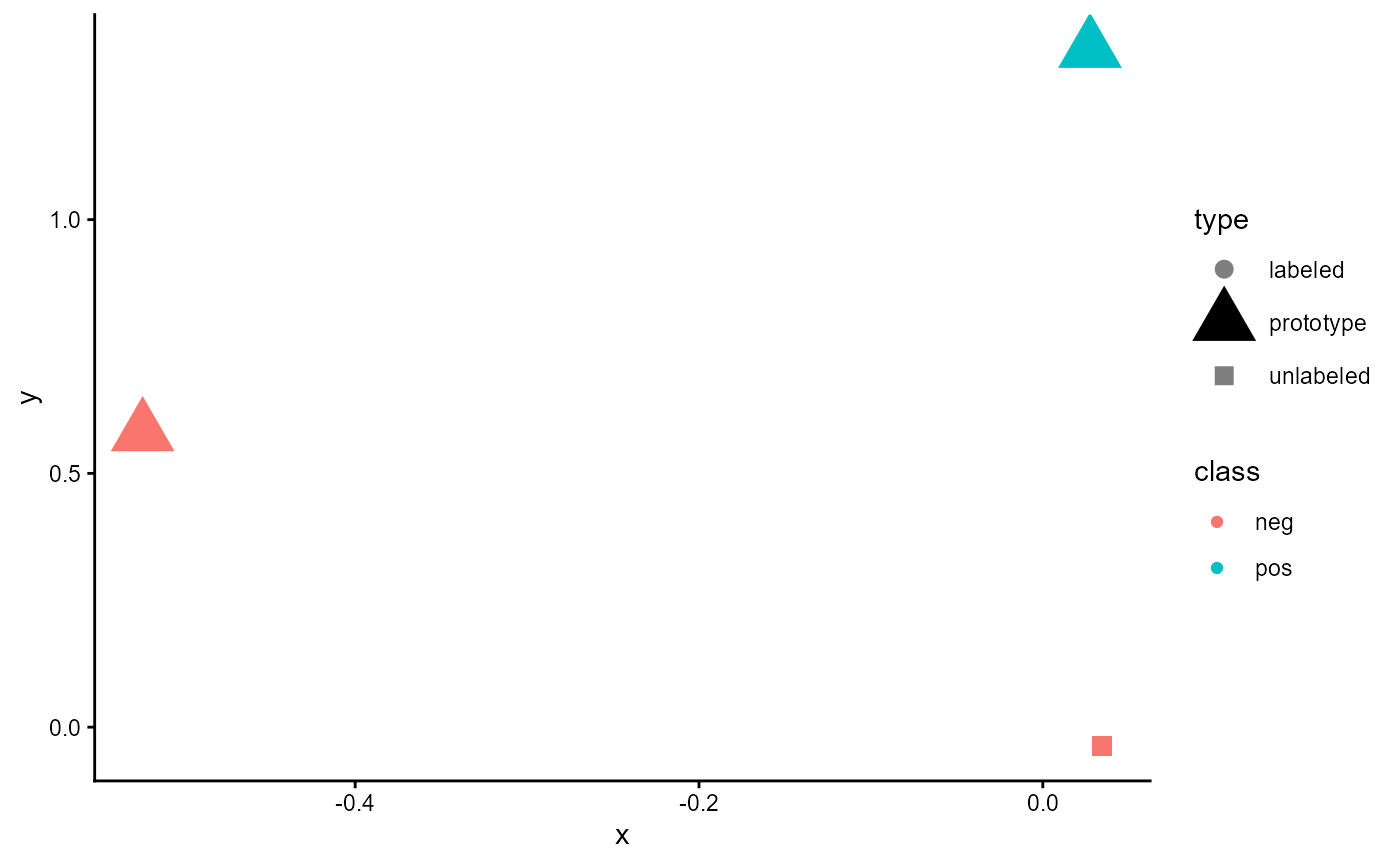
Figure 16: Embeddings of an untrained classifier of type ‘ProtoNet’
The large triangles represent the prototypes for every class while the dots refer to the labeled cases in the data set. For these, the color represents their true class. For unlabeled cases, a square is used. Here, the color indicates the estimated class. As you can see, all cases are located very similarly and there seems to be no clear structure. Let us see how this changes when we train the model.
7.3 Training
classifier_prototype$train(
  data_embeddings = review_embeddings,
  data_targets = review_labels,
  data_folds = 10,
  data_val_size = 0.25,
  loss_pt_fct_name = "MultiWayContrastiveLossFC",
  use_sc = TRUE,
  sc_method = "knnor",
  sc_min_k = 1,
  sc_max_k = 10,
  use_pl = FALSE,
  pl_max_steps = 3,
  pl_max = 1.00,
  pl_anchor = 1.00,
  pl_min = 0.00,
  sustain_track = TRUE,
  sustain_iso_code = "DEU",
  sustain_region = NULL,
  sustain_interval = 15,
  sustain_log_level = "error",
  epochs = 2000,
  batch_size = 32,
  Ns = 18,
  Nq = 3,
  loss_alpha = 0.50,
  loss_margin = 0.05,
  sampling_separate = FALSE,
  sampling_shuffle = TRUE,
  trace = TRUE,
  ml_trace = 0,
  log_dir = NULL,
  log_write_interval = 10,
  n_cores = auto_n_cores(),
  lr_rate = 0.0,
  lr_min = 0.0,
  lr_scheduler = "None",
  lr_warm_up_ratio = 0.05,
  optimizer = "AdamW",
  amp = TRUE
)
#> 2026-07-06 12:17:43 Total Cases: 300 Unique Cases: 300 Labeled Cases: 225
#> 2026-07-06 12:17:45 Start
#> 2026-07-06 12:17:45 Start Sustainability Tracking
#> 2026-07-06 12:17:45 Estimating Learning Rates
#> 2026-07-06 12:19:01 Set lr_rate to 7.5e-02 and lr_min to 7.5e-06.
#> 2026-07-06 12:19:01 | Iteration 1 from 10
#> 2026-07-06 12:19:01 | Iteration 1 from 10 | Generating synthetic cases
#> 2026-07-06 12:19:22 | Iteration 1 from 10 | Generating synthetic cases done
#> 2026-07-06 12:19:22 | Iteration 1 from 10 | Training
#> Data Set Type: Test | ELC: 1973 | Loss 0.1829 | ACC: 0.6818 | BACC: 0.6524 | Avg. Iota: 0.4874 | Smoothed Avg. Iota: 0.3590
#> 2026-07-06 12:31:49 | Iteration 2 from 10
#> 2026-07-06 12:31:49 | Iteration 2 from 10 | Generating synthetic cases
#> 2026-07-06 12:32:12 | Iteration 2 from 10 | Generating synthetic cases done
#> 2026-07-06 12:32:12 | Iteration 2 from 10 | Training
#> Data Set Type: Test | ELC: 858 | Loss 0.0869 | ACC: 0.8636 | BACC: 0.8238 | Avg. Iota: 0.7243 | Smoothed Avg. Iota: 0.3762
#> 2026-07-06 12:44:41 | Iteration 3 from 10
#> 2026-07-06 12:44:41 | Iteration 3 from 10 | Generating synthetic cases
#> 2026-07-06 12:45:01 | Iteration 3 from 10 | Generating synthetic cases done
#> 2026-07-06 12:45:01 | Iteration 3 from 10 | Training
#> Data Set Type: Test | ELC: 1041 | Loss 0.1030 | ACC: 0.9091 | BACC: 0.8952 | Avg. Iota: 0.8125 | Smoothed Avg. Iota: 0.3948
#> 2026-07-06 12:57:28 | Iteration 4 from 10
#> 2026-07-06 12:57:28 | Iteration 4 from 10 | Generating synthetic cases
#> 2026-07-06 12:57:36 | Iteration 4 from 10 | Generating synthetic cases done
#> 2026-07-06 12:57:36 | Iteration 4 from 10 | Training
#> Data Set Type: Test | ELC: 1880 | Loss 0.1093 | ACC: 0.8636 | BACC: 0.8619 | Avg. Iota: 0.7396 | Smoothed Avg. Iota: 0.3828
#> 2026-07-06 13:10:05 | Iteration 5 from 10
#> 2026-07-06 13:10:05 | Iteration 5 from 10 | Generating synthetic cases
#> 2026-07-06 13:10:25 | Iteration 5 from 10 | Generating synthetic cases done
#> 2026-07-06 13:10:25 | Iteration 5 from 10 | Training
#> Data Set Type: Test | ELC: 1914 | Loss 0.1482 | ACC: 0.8636 | BACC: 0.9000 | Avg. Iota: 0.7500 | Smoothed Avg. Iota: 0.3862
#> 2026-07-06 13:22:56 | Iteration 6 from 10
#> 2026-07-06 13:22:56 | Iteration 6 from 10 | Generating synthetic cases
#> 2026-07-06 13:23:17 | Iteration 6 from 10 | Generating synthetic cases done
#> 2026-07-06 13:23:17 | Iteration 6 from 10 | Training
#> Data Set Type: Test | ELC: 811 | Loss 0.2409 | ACC: 0.6957 | BACC: 0.7083 | Avg. Iota: 0.5249 | Smoothed Avg. Iota: 0.3630
#> 2026-07-06 13:35:44 | Iteration 7 from 10
#> 2026-07-06 13:35:44 | Iteration 7 from 10 | Generating synthetic cases
#> 2026-07-06 13:36:10 | Iteration 7 from 10 | Generating synthetic cases done
#> 2026-07-06 13:36:10 | Iteration 7 from 10 | Training
#> Data Set Type: Test | ELC: 1822 | Loss 0.0727 | ACC: 0.9130 | BACC: 0.9042 | Avg. Iota: 0.8264 | Smoothed Avg. Iota: 0.4127
#> 2026-07-06 13:48:38 | Iteration 8 from 10
#> 2026-07-06 13:48:38 | Iteration 8 from 10 | Generating synthetic cases
#> 2026-07-06 13:49:02 | Iteration 8 from 10 | Generating synthetic cases done
#> 2026-07-06 13:49:02 | Iteration 8 from 10 | Training
#> Data Set Type: Test | ELC: 1267 | Loss 0.1268 | ACC: 0.8696 | BACC: 0.8708 | Avg. Iota: 0.7563 | Smoothed Avg. Iota: 0.3848
#> 2026-07-06 14:01:30 | Iteration 9 from 10
#> 2026-07-06 14:01:30 | Iteration 9 from 10 | Generating synthetic cases
#> 2026-07-06 14:01:54 | Iteration 9 from 10 | Generating synthetic cases done
#> 2026-07-06 14:01:54 | Iteration 9 from 10 | Training
#> Data Set Type: Test | ELC: 1980 | Loss 0.1165 | ACC: 0.8696 | BACC: 0.8417 | Avg. Iota: 0.7451 | Smoothed Avg. Iota: 0.3964
#> 2026-07-06 14:14:21 | Iteration 10 from 10
#> 2026-07-06 14:14:21 | Iteration 10 from 10 | Generating synthetic cases
#> 2026-07-06 14:14:42 | Iteration 10 from 10 | Generating synthetic cases done
#> 2026-07-06 14:14:42 | Iteration 10 from 10 | Training
#> Data Set Type: Test | ELC: 685 | Loss 0.0731 | ACC: 0.9130 | BACC: 0.9042 | Avg. Iota: 0.8264 | Smoothed Avg. Iota: 0.3957
#> 2026-07-06 14:27:10 | Final training
#> 2026-07-06 14:27:10 | Final training | Generating synthetic cases
#> 2026-07-06 14:27:39 | Final training | Generating synthetic cases done
#> 2026-07-06 14:27:39 | Final training | Training
#> Data Set Type: Validation | ELC: 778 | Loss 0.1692 | ACC: 0.8909 | BACC: 0.8904 | Avg. Iota: 0.7867 | Smoothed Avg. Iota: 0.4023
#> 2026-07-06 14:42:29 Stop Sustainability Tracking
#> 2026-07-06 14:42:29 Training Complete
While there are no arguments for requesting a balance of the class
weights (loss_balance_class_weights) or balancing the
sequence length (loss_balance_sequence_length), four new
arguments are available. With Ns you determine how many
examples of every class should be used during training within
the support sample. These examples are used to calculate the prototypes
for every class. With Nq you determine how many examples of
every class should be part of the query sample. During training
the network tries to predict the correct classes of query sample.
The arguments loss_alpha and loss_margin
refer to the configuration of the loss function describes by Zhang et
al. (2019). loss_margin refers to the minimal distance all
examples of the query sample should have to all prototypes that do
not represent their class. loss_alpha determines
if the loss should pay more attention to minimize the distance between
the examples to their corresponding prototype or if it should pay more
attention to maximize the distance to the prototypes that do not
represent their class. If you set loss_alpha=1, the loss
tries to minimize the distance of the examples to their corresponding
prototype. If you set loss_alpha=0, loss tries to maximize
the distance of all examples to all prototypes that do not reflect their
class.
The next two important arguments refer to the sampling strategies
during training. With sampling_separate=TRUE, cases for
sample and query a drawn from the same pool of cases. Thus, a specific
case can be a sample case in one epoch and a query case in another
epoch. However, it is ensured that a specific cases never occurs as a
sample and a query case during the same training step.
In addition, it is ensured that every case exists only once during a
training step. If you set sampling_separate=FALSE, the
training data set is split into one data pool for sample and one data
pool for query. Thus, a case can only be a sample case
or query case. With shuffle you can
request that for every training step a random sample is chosen from the
training data set, resulting in different combinations of sample and
query cases. For the training we highly recommend to set
shuffle=TRUE, since this will result in better performing
classifiers.
During training the model generates prototpyes based on all available data and classes of the training data set (sample and query). These classes and prototypes are used for the case that no sample data is provided.
First we plot the analysis of learning rates.
classifier_prototype$plot_learning_rate()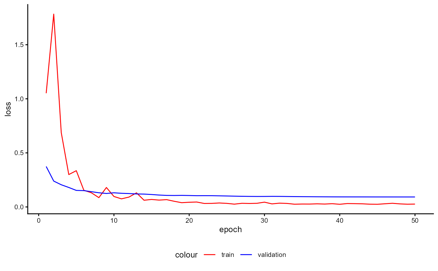
Figure 16: Analysis of Different Learning Rates
Second we plot the training history for the loss and average iota during performance estimation stage.
classifier_prototype$plot_training_history(
  final_training = FALSE,
  pl_step = NULL,
  measure = "loss",
  ind_best_model = FALSE,
  ind_selected_model = TRUE,
  x_min = NULL,
  x_max = NULL,
  y_min = NULL,
  y_max = NULL,
  add_min_max = FALSE,
  text_size = 10
)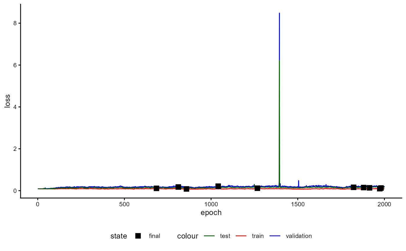
Figure 17: Training History of a Classifier with Prototypes during Performance Estimation Stage (loss)
classifier_prototype$plot_training_history(
  final_training = FALSE,
  pl_step = NULL,
  measure = "avg_iota",
  ind_best_model = FALSE,
  ind_selected_model = TRUE,
  x_min = NULL,
  x_max = NULL,
  y_min = NULL,
  y_max = NULL,
  add_min_max = FALSE,
  text_size = 10
)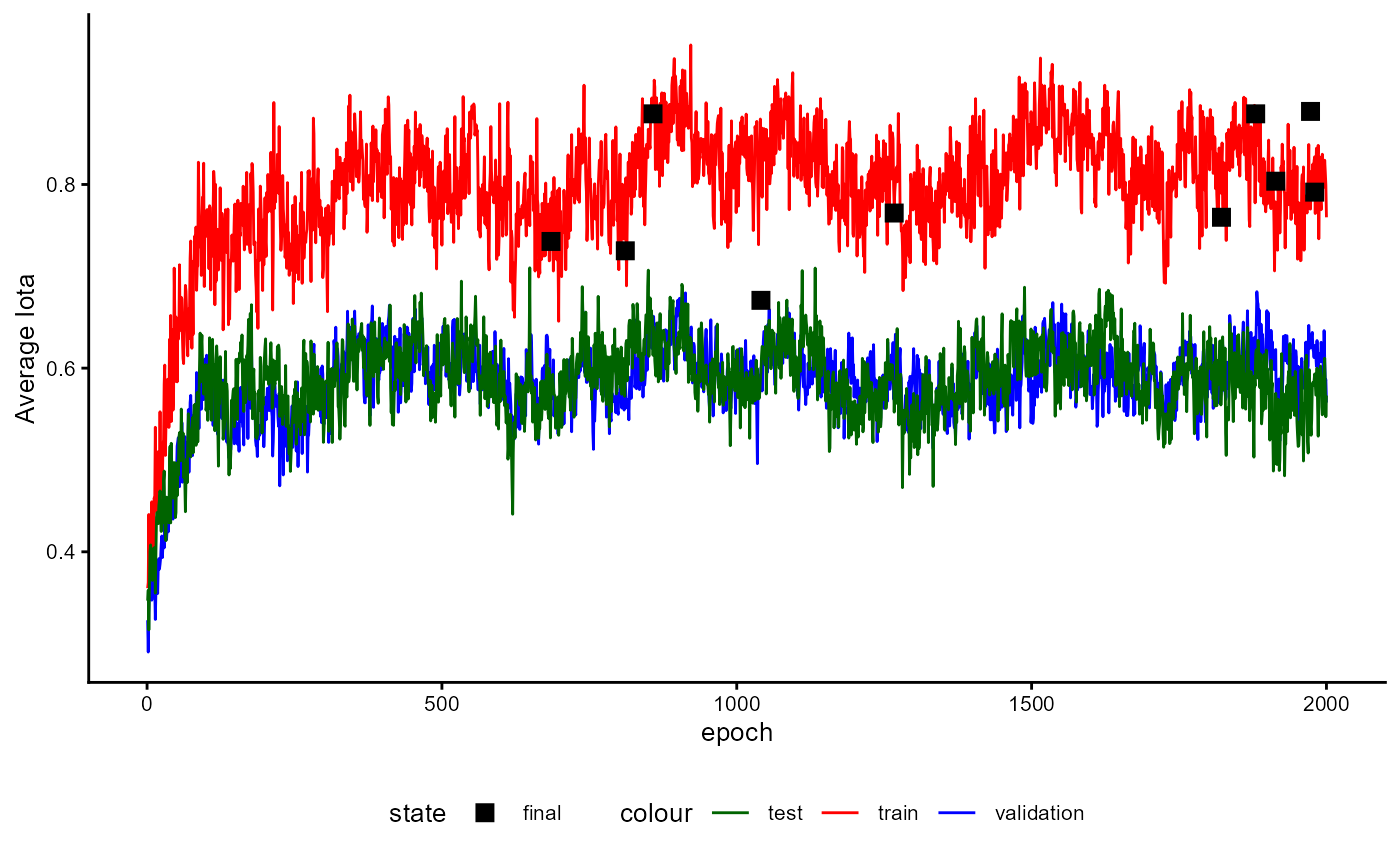
Figure 18: Training History of a Classifier with Prototypes during Performance Estimation Stage (iota)
classifier_prototype$plot_training_history(
  final_training = FALSE,
  pl_step = NULL,
  measure = "s_avg_iota",
  ind_best_model = FALSE,
  ind_selected_model = TRUE,
  x_min = NULL,
  x_max = NULL,
  y_min = NULL,
  y_max = NULL,
  add_min_max = FALSE,
  text_size = 10
)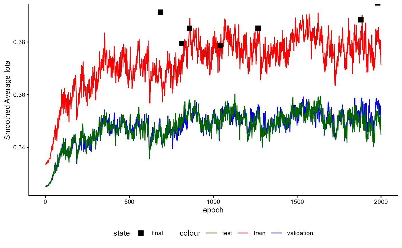
Figure 19: Training History of a Classifier with Prototypes during Performance Estimation Stage (smoothed iota)
The training history of the final training stage is displayed in the following Figures.
classifier_prototype$plot_training_history(
  final_training = TRUE,
  pl_step = NULL,
  measure = "loss",
  ind_best_model = TRUE,
  ind_selected_model = TRUE,
  x_min = NULL,
  x_max = NULL,
  y_min = NULL,
  y_max = NULL,
  add_min_max = FALSE,
  text_size = 10
)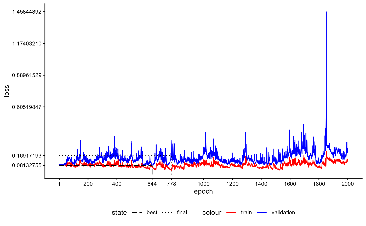
Figure 20: Training History of a Classifier with Prototypes during Final Training Stage (loss)
classifier_prototype$plot_training_history(
  final_training = TRUE,
  pl_step = NULL,
  measure = "avg_iota",
  ind_best_model = FALSE,
  ind_selected_model = TRUE,
  x_min = NULL,
  x_max = NULL,
  y_min = NULL,
  y_max = NULL,
  add_min_max = FALSE,
  text_size = 10
)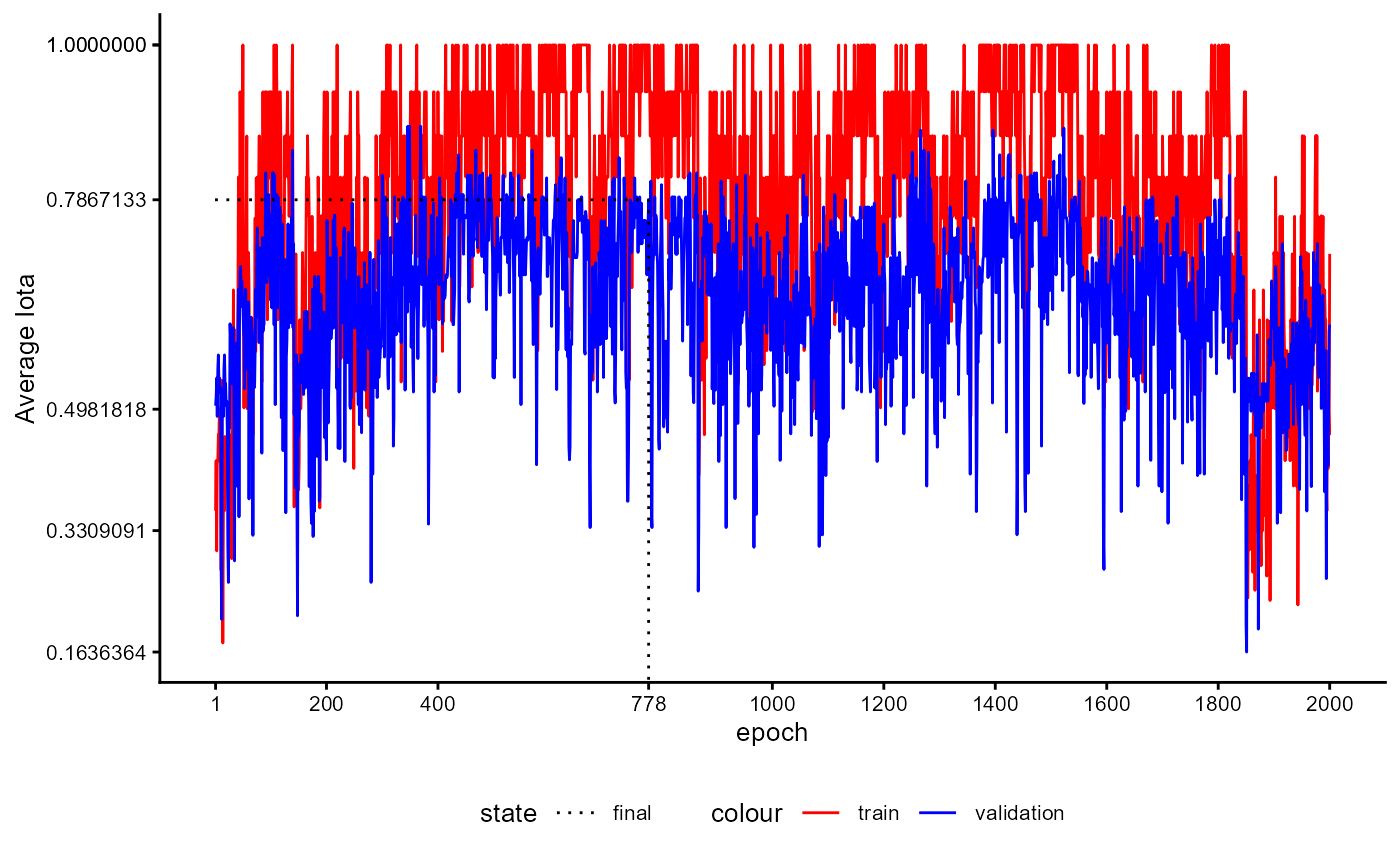
Figure 21: Training History of a Classifier with Prototypes during Final Training Stage (iota)
classifier_prototype$plot_training_history(
  final_training = TRUE,
  pl_step = NULL,
  measure = "s_avg_iota",
  ind_best_model = FALSE,
  ind_selected_model = TRUE,
  x_min = NULL,
  x_max = NULL,
  y_min = NULL,
  y_max = NULL,
  add_min_max = FALSE,
  text_size = 10
)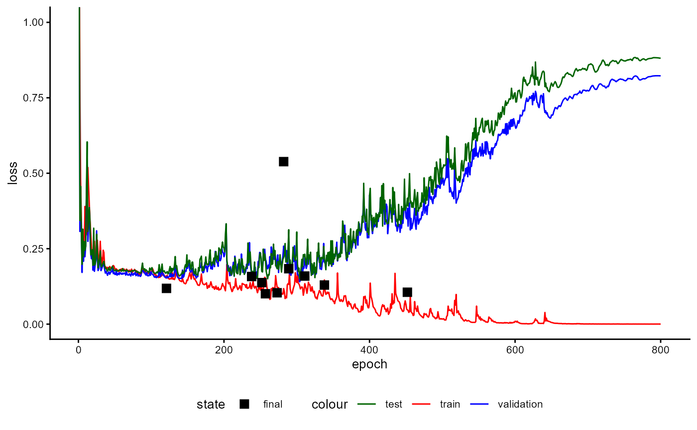
Figure 22: Training History of a Classifier with Prototypes during Final Training Stage (smoothed iota)
After training we can request a visualization of the data again. We
first omit all unlabeled cases by setting
inc_unlabeled=FALSE in order to get an impression of the
quality of training.
plot_trained_1 <- classifier_prototype$plot_embeddings(
  embeddings_q = review_embeddings,
  classes_q = review_labels,
  inc_unlabeled = FALSE
)
plot_trained_1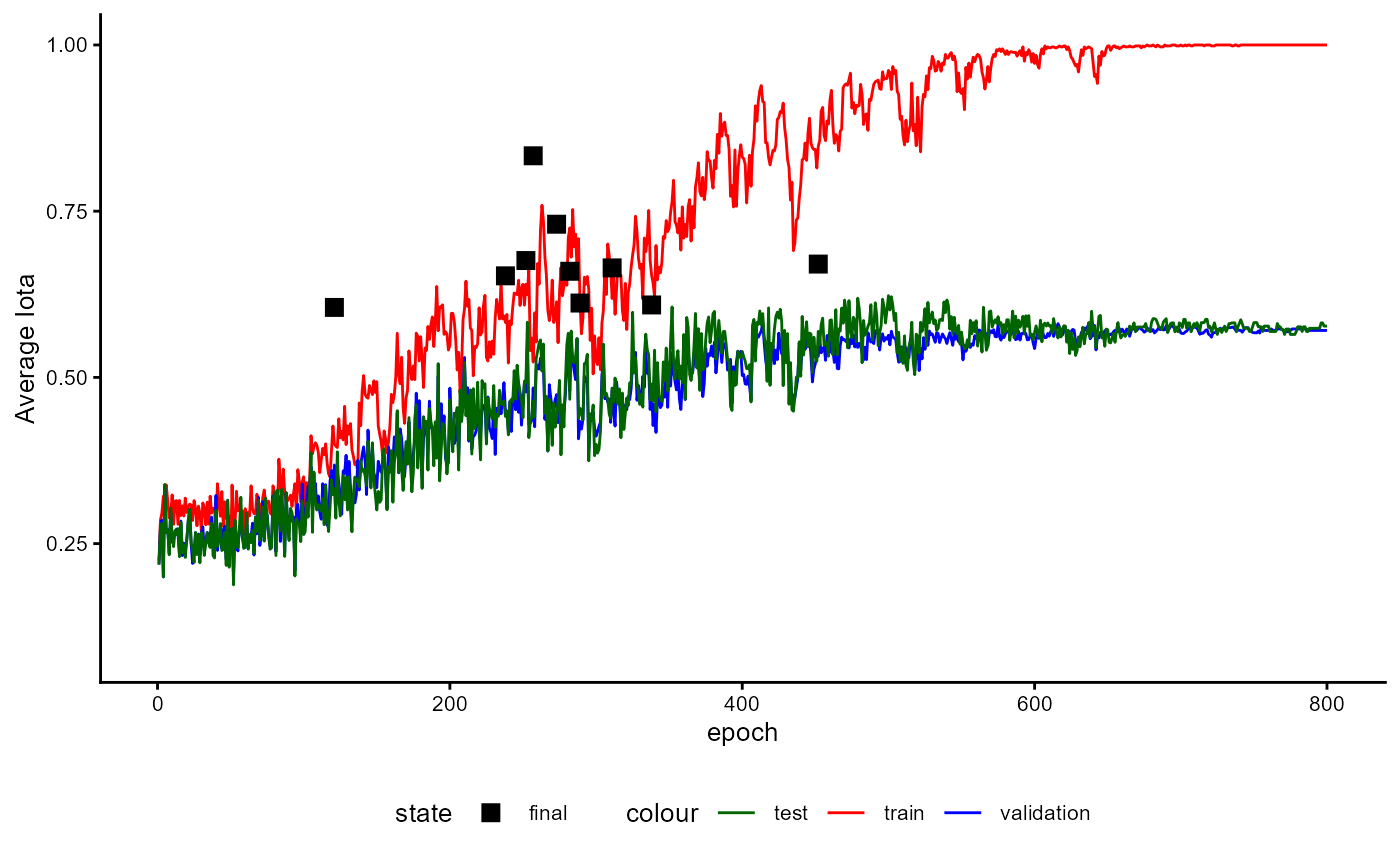
Figure 23: Embeddings of a trained classifier of type ‘ProtoNet’ without unlabeled cases
As shown in the figure, all cases are now sorted. Cases of the class
“neg” are located close to the prototype for “neg”, while cases of the
class “pos” are located near the prototype for “pos”. The black cycle
around the prototypes represent the margin used during training
(loss_margin). Since we use the same data as during
training, this result has to be expected. Only a small number of cases
is located near the wrong prototype. This can be seen if a red dot is
close to the prototype for “pos” and a blue dot is close to the red
prototype for “neg”.
Let us now add the unlabeled cases to the plot by setting
inc_unlabeled=TRUE.
As the following figure shows, the model estimates the class of these cases according to their distance to the two prototypes. Cases that are close to the prototype for “pos” are assigned to “pos”, while cases near the prototype for “neg” are assigned to “neg”.
plot_trained_2 <- classifier_prototype$plot_embeddings(
  embeddings_q = review_embeddings,
  classes_q = review_labels,
  inc_unlabeled = TRUE
)
plot_trained_2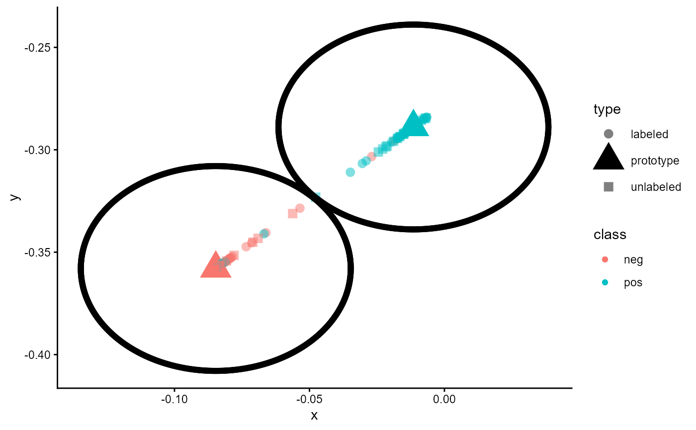
Figure 25: Embedding of a trained classifier of type ‘ProtoNet’ including unlabeled cases
7.4 Performance Evaluation
Finally, let us report the reliability of this classifier.
classifier_prototype$reliability$test_metric_mean
#>           iota_index            min_iota2            avg_iota2
#>            0.6976285            0.6572397            0.7265651
#>            max_iota2            min_alpha            avg_alpha
#>            0.7958905            0.7833333            0.8395833
#>            max_alpha    static_iota_index   dynamic_iota_index
#>            0.8958333            0.3443491            0.6020231
#>       kalpha_nominal       kalpha_ordinal              kendall
#>            0.6744186            0.6744186            0.8371566
#>   c_kappa_unweighted       c_kappa_linear      c_kappa_squared
#>            0.6690065            0.6690065            0.6690065
#>         kappa_fleiss percentage_agreement    balanced_accuracy
#>            0.6670075            0.8488142            0.8395833
#>     gwet_ac1_nominal      gwet_ac2_linear   gwet_ac2_quadratic
#>            0.7221883            0.7221883            0.7221883
#>        avg_precision           avg_recall               avg_f1
#>            0.8354473            0.8395833            0.8335037
classifier_prototype$reliability$standard_measures_mean
#>     precision    recall        f1
#> neg 0.7677994 0.8125000 0.7845488
#> pos 0.9030952 0.8666667 0.8824587
7.5 Application with Sample Data
Up to this point we did not provide sample data. Thus, the model used the classes and prototypes available during training. This is not the regular case for this kind of models. In general, a query and a sample data is given to the classifier. We describe how this works in the following sections.
To illustrate this process, we modify the data from section 2.3. We label some of the positive reviews as “very positive” and some of the negative reviews as “very negative”. Thus, we increase the number of classes/categories from 2 to 4.
example_data <- imdb_movie_reviews
example_data$label <- as.character(example_data$label)
example_data$label[c(1:15)] <- "very negative"
example_data$label[c(76:100)] <- NA
example_data$label[c(201:250)] <- NA
example_data$label[c(251:260)] <- "very positive"
example_data$label <- factor(example_data$label)
table(example_data$label, useNA = "ifany")
#>
#>           neg           pos very negative very positive          <NA>
#>            60           140            15            10            75
Our aim is now to predict the 75 cases with no labels with the help of our trained model although the model was trained only for two and different classes. Thus, we first have to split the data. The cases with classes/categories form the sample set and the cases without any classes/categories form the query set.
sample_set_raw <- subset(example_data, !is.na(example_data$label))
sample_classes <- sample_set_raw$label
table(sample_classes, useNA = "ifany")
#> sample_classes
#>           neg           pos very negative very positive
#>            60           140            15            10

sample_texts <- LargeDataSetForText$new()
sample_texts$add_from_data.frame(sample_set_raw)
query_set_raw <- subset(example_data, is.na(example_data$label))
table(query_set_raw$label, useNA = "ifany")
#>
#>           neg           pos very negative very positive          <NA>
#>             0             0             0             0            75

query_texts <- LargeDataSetForText$new()
query_texts$add_from_data.frame(query_set_raw)
Now we must create text embeddings for the query and the sample data set. We have to use the same embedding model as we used during training the classifier.
sample_embeddings <- tem$embed_large(
  text_dataset = sample_texts,
  trace = TRUE
)
#> Calculating Embeddings  12.50 % (1|8) done ETA: 0000::00::11Calculating Embeddings  25.00 % (2|8) done ETA: 0000::00::09Calculating Embeddings  37.50 % (3|8) done ETA: 0000::00::07Calculating Embeddings  50.00 % (4|8) done ETA: 0000::00::06Calculating Embeddings  62.50 % (5|8) done ETA: 0000::00::04Calculating Embeddings  75.00 % (6|8) done ETA: 0000::00::03Calculating Embeddings  87.50 % (7|8) done ETA: 0000::00::01Calculating Embeddings  100.00 % (8|8) done ETA: 0000::00::00
query_embeddings <- tem$embed_large(
  text_dataset = query_texts,
  trace = TRUE
)
#> Calculating Embeddings  33.33 % (1|3) done ETA: 0000::00::02Calculating Embeddings  66.67 % (2|3) done ETA: 0000::00::01Calculating Embeddings  100.00 % (3|3) done ETA: 0000::00::00
Now we are ready to use our classifier. First, we predict the classes of the query sample.
new_predictions <- classifier_prototype$predict_with_samples(
  newdata = query_embeddings,
  embeddings_s = sample_embeddings,
  classes_s = sample_classes
)
head(new_predictions)
#>            neg       pos very negative very positive expected_category
#> 8016 0.3024086 0.1941184     0.3099263     0.1935467     very negative
#> 9118 0.2664179 0.2366553     0.2611826     0.2357443               neg
#> 6376 0.3023873 0.1941383     0.3099076     0.1935668     very negative
#> 5766 0.3024555 0.1940646     0.3099873     0.1934925     very negative
#> 5942 0.3024316 0.1940917     0.3099569     0.1935197     very negative
#> 478  0.3083823 0.1956987     0.3008225     0.1950965               neg
table(new_predictions$expected_category)
#>
#>           neg           pos very negative very positive
#>             6            10            16            43
Although we trained our classifier for two classes we can now use it to predict other classes. Next, we plot the results.
plot_with_samples <- classifier_prototype$plot_embeddings(
  embeddings_q = query_embeddings,
  embeddings_s = sample_embeddings,
  classes_s = sample_classes,
  inc_unlabeled = TRUE,
  inc_margin = FALSE
)
plot_with_samples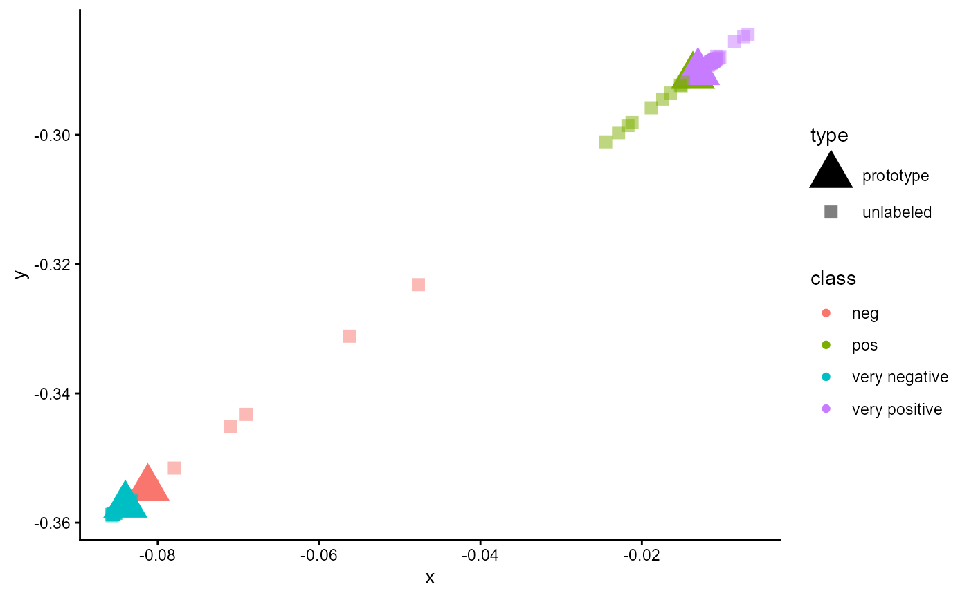
Figure 26: Embeddings of a trained classifier of type ‘ProtoNet’ trained for two classes and applied for a sample set with four classes.
8 Feature Extractors
8.1 Introduction
Another option to increase a model’s performance and/or to increase computational speed is to apply a feature extractor. For example, the work by Ganesan et al. (2021) indicates that a reduction of the hidden size can increase a model’s accuracy. In aifeducation, a feature extractor is a model that tries to reduce the number of features of given text embeddings before feeding the embeddings as input to a classifier.
The feature extractors implemented in aifeducation are auto-encoders that support sequential data and sequences of different length. The basic architecture of all extractors is shown in the following figure.
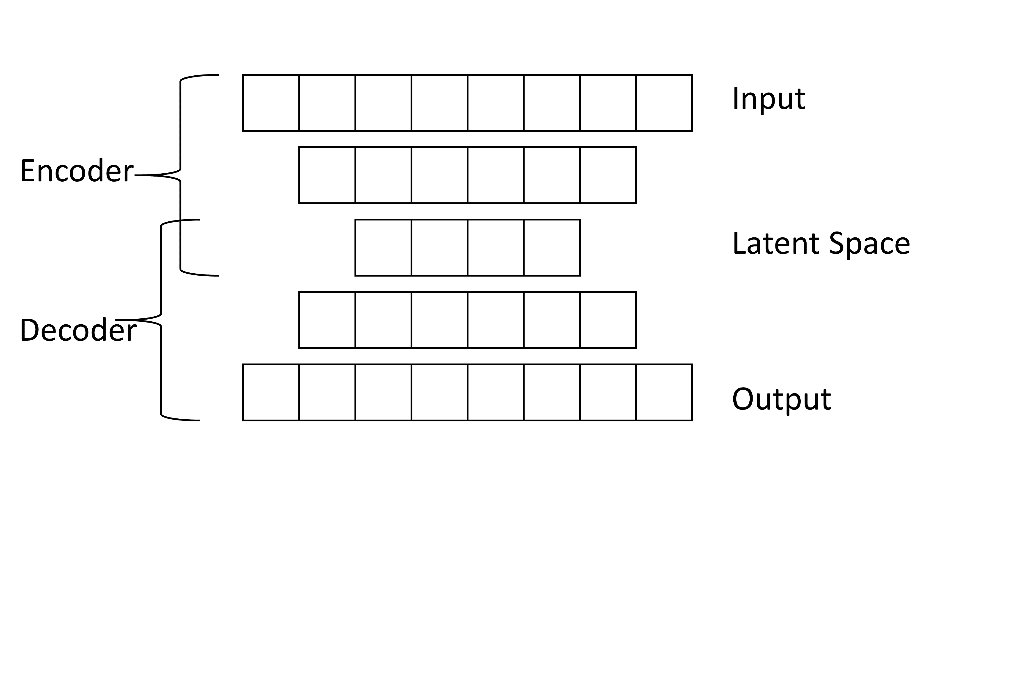
The learning objective of the feature extractors is first to compress information by reducing the number of features to the number of features of the latent space (Frochte 2019, p.281). In the figure above, this would mean to reduce the number of features from 8 to 4 and to store as much information as possible from the 8 dimensions in only 4 dimensions. In the next step, the extractor tries to reconstruct the original information from the compressed information of the latent space (Frochte 2019, pp.280-281). The information is extended from 4 dimensions to 8. After training, the hidden representation of the latent space is used as a compression of the original input.
8.2 Creation
You can create a feature extractor as follows. In this example we use the text embeddings from section 4.
feature_extractor <- TEFeatureExtractor$new()
feature_extractor$configure(
  name = "feature_extractor_bert_movie_reviews",
  label = "Feature extractor for Text Embeddings",
  text_embeddings = review_embeddings,
  features = 384,
  method = "Dense",
  orthogonal_method = "matrix_exp",
  noise_factor = 0.0
)
Similarly to the other models, you can use label for the
model’s label. The argument text_embeddings takes an object
of class EmbeddedText or
LargeDataSetForTextEmbeddings. With this object you connect
your feature extractor with a specific TextEmbeddingModel. That is, the
feature extractor works only with embeddings from exactly the same
TextEmbeddingModel.
features determines the number of features for the
compressed representation. The lower the number, the higher the
requested compression. This value corresponds to the features of the
latent space in the figure above.
You should use this value depending on the number of features of the
underlying text embedding model. You can request this value by calling
the method get_n_features like this:
tem$get_n_features()
#> [1] 768
A study by Takeshita et al. (2025) shows that randomly dropping 50% of the dimensions leads only to a minor drop in performance in classification tasks. Thus, this value can serve as a rule of thumb for determining this parameter. Thus we reduce the number of features to 50 % or to 384.
With method you determine the type of layer the feature
extractor should use. If set method="LSTM", all layers of
the model are long short-term memory layers. If set
method="Dense" all layers are standard dense layers.
Independently from your choice, all models try to generate the latent
space such that the co-variance of the features to be zero. Thus, all
features represent unique information. In addition, all methods except
"LSTM" use an orthogonal parameterization to prevent
over-fitting and apply parameter sharing. The opposite layers use the
same parameters. For more details please refer to Ranjan (2019).
With noise_factor you can add some noise during training
making the feature extractor perform a denoising auto-encoder, which can
provide more robust generalizations.
8.3 Training
Training the extractor is identical to the other models in
aifeducation. Please note that the text embeddings provided to
data_embeddings must be generated with the same
TextEmbeddingModel as the embeddings provided during the
configuration of your model.
feature_extractor$train(
  data_embeddings = review_embeddings,
  data_val_size = 0.25,
  sustain_track = TRUE,
  sustain_iso_code = "DEU",
  sustain_region = NULL,
  sustain_interval = 15,
  sustain_log_level = "error",
  epochs = 3000,
  batch_size = 64,
  lr_rate = 0.0,
  lr_min = 0.0,
  lr_scheduler = "None",
  trace = TRUE,
  ml_trace = 0,
  optimizer = "AdamW",
  amp = TRUE,
  lr_warm_up_ratio = 0.10
)
#> 2026-07-06 14:42:52 Start
#> 2026-07-06 14:42:52 Start Sustainability Tracking
#> 2026-07-06 14:42:52 Estimating Learning Rates
#> 2026-07-06 14:44:10 Set lr_rate to 1e-04 and lr_min to 2.5e-06.
#> 2026-07-06 14:56:26 Stop Sustainability Tracking
#> 2026-07-06 14:56:26 Training finished
In this example we use the same text embeddings as we use to train the classifier. It can be beneficial if you use a larger sample of texts for training a
TEFeatureExtractorto improve performance and/or to allow a broad application of the feature extractor.
feature_extractor$plot_learning_rate()
Figure 27: Analysis of Different Learning Rates
You can plot the training history of the model with:
feature_extractor$plot_training_history(
  ind_best_model = TRUE
)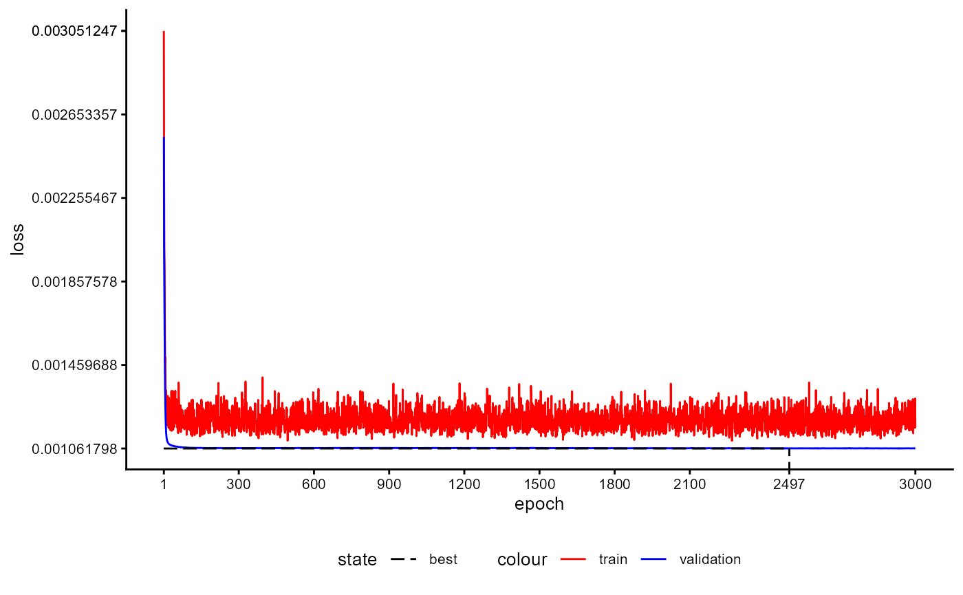
Figure 28: Training History of a Feature Extractor.
You receive a short summary of the extractor by calling
print.
print(feature_extractor)
#> Object      : TEFeatureExtractor
#> ID          : feature_extractor_bert_movie_reviews
#> Label       : Feature extractor for Text Embeddings
#> Configured  : TRUE
#> Trained     : TRUE
#> Times       : 3
#> Features In : 768
#> Features Out: 384
#> Parameter   : 966656
8.4 Application
After you have trained your feature extractor, you can use it for
every classifier. Just pass the feature extractor to
feature_extractor during configuration of the classifier.
Please note that you now have to set the values for
feat_size and cls_pooling_features depending
on the number of features of the feature extractor and not
depending on the number of features of the text embedding model since
the aim of the feature extractor is to reduce this number.
feat_size should be equal or less the number for features
of the feature extractor and cls_pooling_features should be
equal or less the value for feat_size. For the classifier
described in section 6 this would look like:
classifier_with_fe <- TEClassifierSequential$new()
classifier_with_fe$configure(
  label = "Classifier for Estimating a Postive or Negative Rating of Movie Reviews",
  text_embeddings = review_embeddings,
  feature_extractor = feature_extractor,
  target_levels = c("neg", "pos"),
  skip_connection_type = "ResidualGate",
  cls_pooling_features = 20,
  cls_pooling_type = "MaxTimes",
  cls_head_type = "Regular",
  feat_act_fct = "Tanh",
  feat_size = 384,
  feat_bias = TRUE,
  feat_dropout = 0.0,
  feat_parametrizations = "None",
  feat_normalization_type = "PowerNorm",
  ng_conv_act_fct = "GELU",
  ng_conv_n_layers = 1,
  ng_conv_ks_min = 2,
  ng_conv_ks_max = max_chunks,
  ng_conv_bias = FALSE,
  ng_conv_dropout = 0.05,
  ng_conv_parametrizations = "None",
  ng_conv_normalization_type = "PowerNorm",
  ng_conv_residual_type = "ResidualGate",
  dense_act_fct = "GELU",
  dense_n_layers = 2,
  dense_dropout = 0.30,
  dense_bias = FALSE,
  dense_parametrizations = "None",
  dense_normalization_type = "PowerNorm",
  dense_residual_type = "ResidualGate",
  rec_act_fct = "Tanh",
  rec_n_layers = 0,
  rec_type = "GRU",
  rec_bidirectional = FALSE,
  rec_dropout = 0.2,
  rec_bias = FALSE,
  rec_parametrizations = "None",
  rec_normalization_type = "PowerNorm",
  rec_residual_type = "ResidualGate",
  tf_act_fct = "SwiGLU",
  tf_dense_dim = ceiling(2.67 * 64),
  tf_n_layers = 0,
  tf_dropout_rate_1 = 0.1,
  tf_dropout_rate_2 = 0.3,
  tf_attention_type = "MultiHead",
  tf_positional_type = "absolute",
  tf_num_heads = 12,
  tf_bias = FALSE,
  tf_parametrizations = "None",
  tf_normalization_type = "PowerNorm",
  tf_normalization_position = "Pre",
  tf_residual_type = "ResidualGate"
)
That is all. Now you can use and train the classifier in the same way as you did without a feature extractor. You even do not need to save and load the feature extractor manually. This is done automatically for all classifiers.
classifier_with_fe$train(
  data_embeddings = review_embeddings,
  data_targets = review_labels,
  data_folds = 10,
  data_val_size = 0.25,
  loss_balance_class_weights = TRUE,
  loss_balance_sequence_length = TRUE,
  loss_cls_fct_name = "FocalLoss",
  use_sc = TRUE,
  sc_method = "knnor",
  sc_min_k = 1,
  sc_max_k = 10,
  use_pl = FALSE,
  pl_max_steps = 3,
  pl_max = 1.00,
  pl_anchor = 1.00,
  pl_min = 0.00,
  sustain_track = TRUE,
  sustain_iso_code = "DEU",
  sustain_region = NULL,
  sustain_interval = 15,
  sustain_log_level = "error",
  epochs = 4000,
  batch_size = 32,
  trace = TRUE,
  ml_trace = 0,
  log_dir = NULL,
  log_write_interval = 10,
  n_cores = auto_n_cores(),
  lr_rate = 0.0,
  lr_min = 0.0,
  lr_scheduler = "None",
  lr_warm_up_ratio = 0.05,
  optimizer = "AdamW",
  amp = TRUE
)
#> Compress Embeddings  10.00 % (1|10) done ETA: 0000::00::02Compress Embeddings  20.00 % (2|10) done ETA: 0000::00::03Compress Embeddings  30.00 % (3|10) done ETA: 0000::00::02Compress Embeddings  40.00 % (4|10) done ETA: 0000::00::02Compress Embeddings  50.00 % (5|10) done ETA: 0000::00::02Compress Embeddings  60.00 % (6|10) done ETA: 0000::00::02Compress Embeddings  70.00 % (7|10) done ETA: 0000::00::01Compress Embeddings  80.00 % (8|10) done ETA: 0000::00::01Compress Embeddings  90.00 % (9|10) done ETA: 0000::00::00Compress Embeddings  100.00 % (10|10) done ETA: 0000::00::00
#> 2026-07-06 14:56:31 Total Cases: 300 Unique Cases: 300 Labeled Cases: 225
#> 2026-07-06 14:56:34 Start
#> 2026-07-06 14:56:34 Start Sustainability Tracking
#> 2026-07-06 14:56:34 Estimating Learning Rates
#> integer(0)
#> 2026-07-06 14:57:13 Set lr_rate to 7.5e-04 and lr_min to 2.5e-05.
#> 2026-07-06 14:57:13 | Iteration 1 from 10
#> 2026-07-06 14:57:13 | Iteration 1 from 10 | Generating synthetic cases
#> 2026-07-06 14:57:21 | Iteration 1 from 10 | Generating synthetic cases done
#> 2026-07-06 14:57:21 | Iteration 1 from 10 | Training
#> integer(0)
#> Data Set Type: Test | ELC: 3512 | Loss 0.0105 | ACC: 0.7273 | BACC: 0.6095 | Avg. Iota: 0.4750 | Smoothed Avg. Iota: 0.4317
#> 2026-07-06 15:04:41 | Iteration 2 from 10
#> 2026-07-06 15:04:41 | Iteration 2 from 10 | Generating synthetic cases
#> 2026-07-06 15:04:55 | Iteration 2 from 10 | Generating synthetic cases done
#> 2026-07-06 15:04:55 | Iteration 2 from 10 | Training
#> integer(0)
#> Data Set Type: Test | ELC: 3995 | Loss 0.0057 | ACC: 0.8182 | BACC: 0.7524 | Avg. Iota: 0.6389 | Smoothed Avg. Iota: 0.5479
#> 2026-07-06 15:11:28 | Iteration 3 from 10
#> 2026-07-06 15:11:28 | Iteration 3 from 10 | Generating synthetic cases
#> 2026-07-06 15:11:42 | Iteration 3 from 10 | Generating synthetic cases done
#> 2026-07-06 15:11:42 | Iteration 3 from 10 | Training
#> integer(0)
#> Data Set Type: Test | ELC: 3811 | Loss 0.0239 | ACC: 0.6818 | BACC: 0.6143 | Avg. Iota: 0.4658 | Smoothed Avg. Iota: 0.4448
#> 2026-07-06 15:18:13 | Iteration 4 from 10
#> 2026-07-06 15:18:13 | Iteration 4 from 10 | Generating synthetic cases
#> 2026-07-06 15:18:29 | Iteration 4 from 10 | Generating synthetic cases done
#> 2026-07-06 15:18:29 | Iteration 4 from 10 | Training
#> integer(0)
#> Data Set Type: Test | ELC: 3974 | Loss 0.0123 | ACC: 0.7727 | BACC: 0.7190 | Avg. Iota: 0.5833 | Smoothed Avg. Iota: 0.4300
#> 2026-07-06 15:24:57 | Iteration 5 from 10
#> 2026-07-06 15:24:57 | Iteration 5 from 10 | Generating synthetic cases
#> 2026-07-06 15:25:12 | Iteration 5 from 10 | Generating synthetic cases done
#> 2026-07-06 15:25:12 | Iteration 5 from 10 | Training
#> integer(0)
#> Data Set Type: Test | ELC: 3825 | Loss 0.0046 | ACC: 0.8182 | BACC: 0.7905 | Avg. Iota: 0.6601 | Smoothed Avg. Iota: 0.4618
#> 2026-07-06 15:31:40 | Iteration 6 from 10
#> 2026-07-06 15:31:40 | Iteration 6 from 10 | Generating synthetic cases
#> 2026-07-06 15:31:52 | Iteration 6 from 10 | Generating synthetic cases done
#> 2026-07-06 15:31:52 | Iteration 6 from 10 | Training
#> integer(0)
#> Data Set Type: Test | ELC: 752 | Loss 0.0073 | ACC: 0.6957 | BACC: 0.5917 | Avg. Iota: 0.4444 | Smoothed Avg. Iota: 0.3556
#> 2026-07-06 15:38:57 | Iteration 7 from 10
#> 2026-07-06 15:38:57 | Iteration 7 from 10 | Generating synthetic cases
#> 2026-07-06 15:39:11 | Iteration 7 from 10 | Generating synthetic cases done
#> 2026-07-06 15:39:11 | Iteration 7 from 10 | Training
#> integer(0)
#> Data Set Type: Test | ELC: 2621 | Loss 0.0082 | ACC: 0.6522 | BACC: 0.5583 | Avg. Iota: 0.4095 | Smoothed Avg. Iota: 0.4352
#> 2026-07-06 15:45:39 | Iteration 8 from 10
#> 2026-07-06 15:45:39 | Iteration 8 from 10 | Generating synthetic cases
#> 2026-07-06 15:45:54 | Iteration 8 from 10 | Generating synthetic cases done
#> 2026-07-06 15:45:54 | Iteration 8 from 10 | Training
#> integer(0)
#> Data Set Type: Test | ELC: 3683 | Loss 0.0048 | ACC: 0.9130 | BACC: 0.8750 | Avg. Iota: 0.8162 | Smoothed Avg. Iota: 0.4663
#> 2026-07-06 15:52:22 | Iteration 9 from 10
#> 2026-07-06 15:52:22 | Iteration 9 from 10 | Generating synthetic cases
#> 2026-07-06 15:52:37 | Iteration 9 from 10 | Generating synthetic cases done
#> 2026-07-06 15:52:37 | Iteration 9 from 10 | Training
#> integer(0)
#> Data Set Type: Test | ELC: 3411 | Loss 0.0088 | ACC: 0.7391 | BACC: 0.6542 | Avg. Iota: 0.5167 | Smoothed Avg. Iota: 0.5013
#> 2026-07-06 15:59:09 | Iteration 10 from 10
#> 2026-07-06 15:59:09 | Iteration 10 from 10 | Generating synthetic cases
#> 2026-07-06 15:59:24 | Iteration 10 from 10 | Generating synthetic cases done
#> 2026-07-06 15:59:24 | Iteration 10 from 10 | Training
#> integer(0)
#> Data Set Type: Test | ELC: 3444 | Loss 0.0043 | ACC: 0.8261 | BACC: 0.7500 | Avg. Iota: 0.6447 | Smoothed Avg. Iota: 0.5123
#> 2026-07-06 16:06:02 | Final training
#> 2026-07-06 16:06:02 | Final training | Generating synthetic cases
#> 2026-07-06 16:06:11 | Final training | Generating synthetic cases done
#> 2026-07-06 16:06:11 | Final training | Training
#> integer(0)
#> Data Set Type: Validation | ELC: 3988 | Loss 0.0039 | ACC: 0.8545 | BACC: 0.8206 | Avg. Iota: 0.7143 | Smoothed Avg. Iota: 0.5568
#> 2026-07-06 16:13:06 Stop Sustainability Tracking
#> 2026-07-06 16:13:06 Training Complete
First we can analyze the training history of the performance estimation stage.
classifier_with_fe$plot_training_history(
  final_training = FALSE,
  pl_step = NULL,
  measure = "loss",
  ind_best_model = FALSE,
  ind_selected_model = TRUE,
  x_min = NULL,
  x_max = NULL,
  y_min = NULL,
  y_max = 1,
  add_min_max = FALSE,
  text_size = 10
)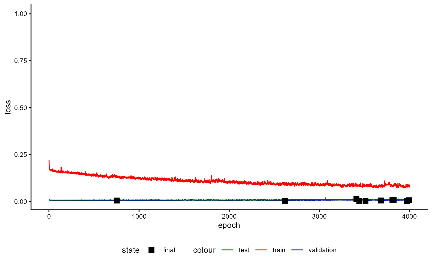
Figure 29: Training History of a Classifier with Feature Extractor during Performance Estimation Stage (loss)
classifier_with_fe$plot_training_history(
  final_training = FALSE,
  pl_step = NULL,
  measure = "avg_iota",
  ind_best_model = FALSE,
  ind_selected_model = TRUE,
  x_min = NULL,
  x_max = NULL,
  y_min = NULL,
  y_max = NULL,
  add_min_max = FALSE,
  text_size = 10
)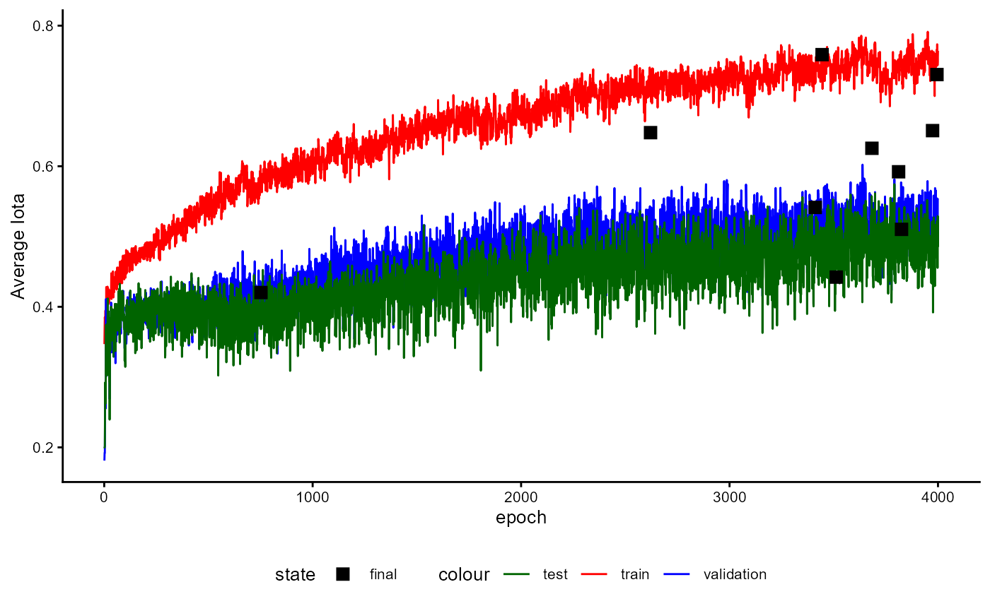
Figure 30: Training History of a Classifier with Feature Extractor during Performance Estimation Stage (iota)
classifier_with_fe$plot_training_history(
  final_training = FALSE,
  pl_step = NULL,
  measure = "s_avg_iota",
  ind_best_model = FALSE,
  ind_selected_model = TRUE,
  x_min = NULL,
  x_max = NULL,
  y_min = NULL,
  y_max = NULL,
  add_min_max = FALSE,
  text_size = 10
)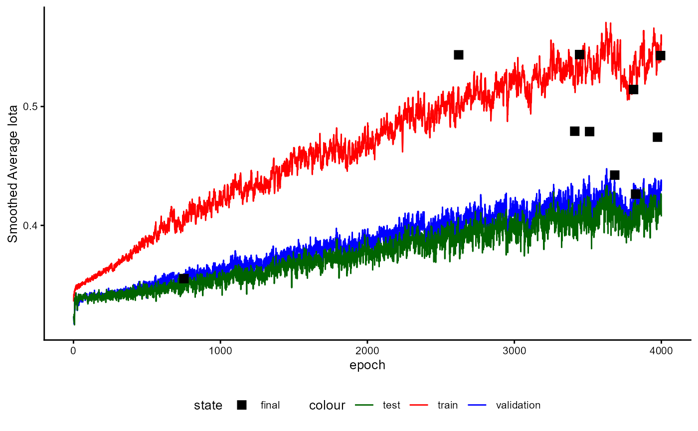
Figure 31: Training History of a Classifier with Feature Extractor during Performance Estimation Stage (smoothed iota)
The training history of the final training stage is displayed in the following two Figures.
classifier_with_fe$plot_training_history(
  final_training = TRUE,
  pl_step = NULL,
  measure = "loss",
  ind_best_model = FALSE,
  ind_selected_model = TRUE,
  x_min = NULL,
  x_max = NULL,
  y_min = NULL,
  y_max = 1,
  add_min_max = FALSE,
  text_size = 10
)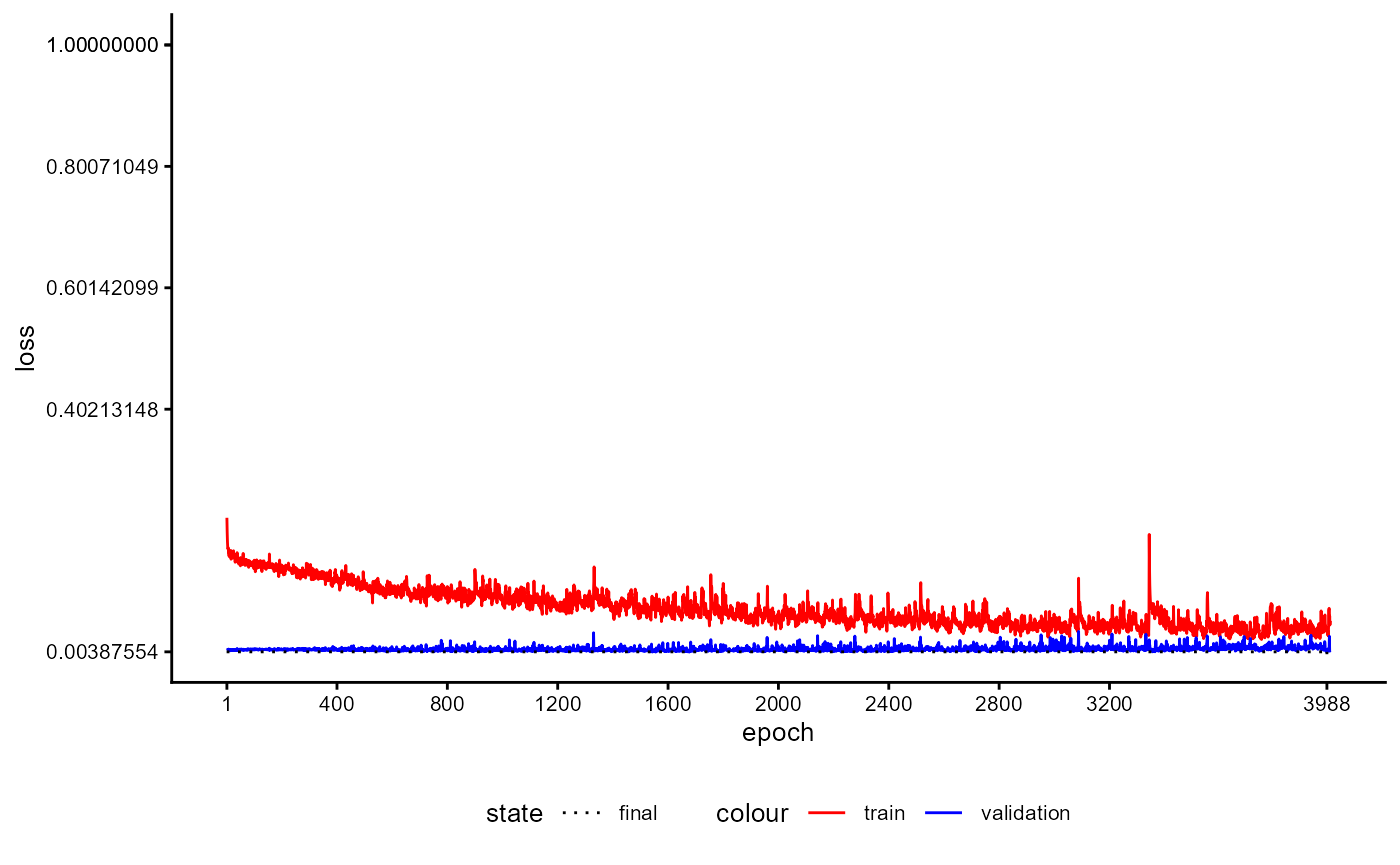
Figure 32: Training History of a Classifier with Feature Extractor during Final Training Stage (loss)
classifier_with_fe$plot_training_history(
  final_training = TRUE,
  pl_step = NULL,
  measure = "avg_iota",
  ind_best_model = FALSE,
  ind_selected_model = TRUE,
  x_min = NULL,
  x_max = NULL,
  y_min = NULL,
  y_max = NULL,
  add_min_max = FALSE,
  text_size = 10
)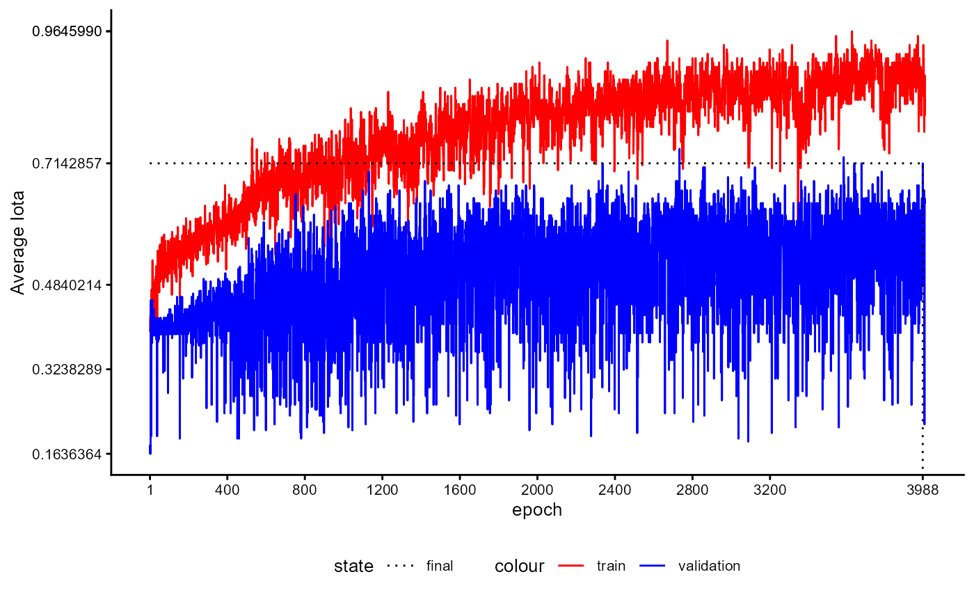
Figure 33: Training History of a Classifier with Feature Extractor during Final Training Stage (iota)
classifier_with_fe$plot_training_history(
  final_training = TRUE,
  pl_step = NULL,
  measure = "s_avg_iota",
  ind_best_model = FALSE,
  ind_selected_model = TRUE,
  x_min = NULL,
  x_max = NULL,
  y_min = NULL,
  y_max = NULL,
  add_min_max = FALSE,
  text_size = 10
)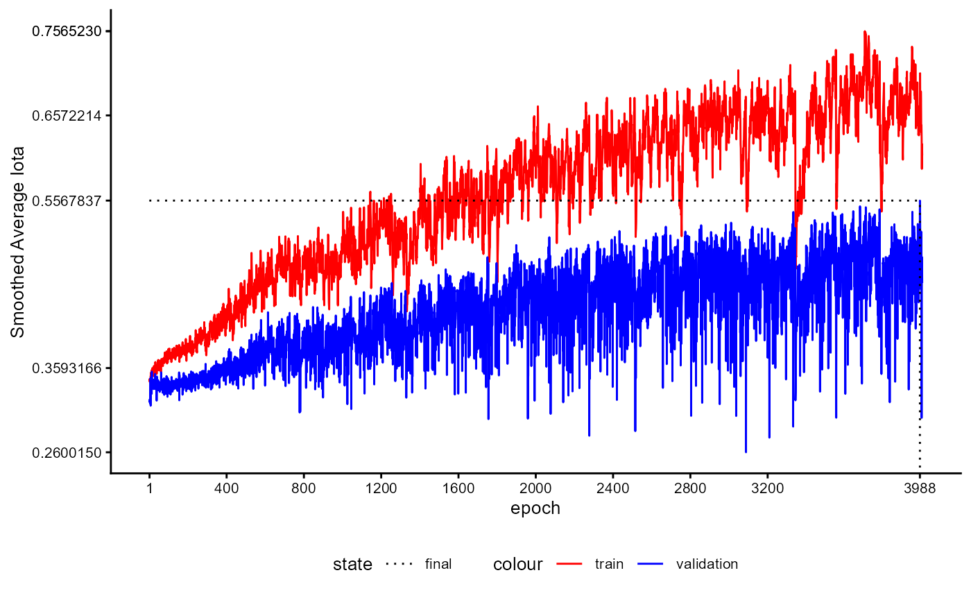
Figure 34: Training History of a Classifier with Feature Extractor during Final Training Stage (smoothed iota)
For example, let us explore the performance of the classifier.
classifier_with_fe$reliability$test_metric_mean
#>           iota_index            min_iota2            avg_iota2
#>            0.5905138            0.4055556            0.5654691
#>            max_iota2            min_alpha            avg_alpha
#>            0.7253826            0.4696429            0.6914881
#>            max_alpha    static_iota_index   dynamic_iota_index
#>            0.9133333            0.3513623            0.4974252
#>       kalpha_nominal       kalpha_ordinal              kendall
#>            0.4098970            0.4098970            0.7153612
#>   c_kappa_unweighted       c_kappa_linear      c_kappa_squared
#>            0.4137105            0.4137105            0.4137105
#>         kappa_fleiss percentage_agreement    balanced_accuracy
#>            0.3964842            0.7644269            0.6914881
#>     gwet_ac1_nominal      gwet_ac2_linear   gwet_ac2_quadratic
#>            0.6119446            0.6119446            0.6119446
#>        avg_precision           avg_recall               avg_f1
#>            0.7523352            0.6914881            0.6982421
classifier_with_fe$reliability$standard_measures_mean
#>     precision    recall        f1
#> neg 0.7264286 0.4696429 0.5578655
#> pos 0.7782417 0.9133333 0.8386188
8.5. Saving and Loading
If you would like to save and load a TEFeatureExtractor
independently from a classifier you can use the function pair
save_to_disk and load_from_disk as with the
other objects of this package. This is useful if you would like to use
the TEFeatureExtractor at a later time point in combination
with other models.
9 Plots for Training History
9.1 BaseModels
BaseModels, TEFeatureExtractors, and classifiers allow you to create plots showing your model’s training process. The process of requesting these plots is similar for all objects. However, classifiers offer the greatest degree of customization of graphics. This chapter shows you how to use the plots. We refer to the models from previous chapters to provide some examples.
We start with the base models. Thex_min,
x_max, y_min, and y_max arguments
allow you to zoom in or out. If you set these arguments to
NULL, the values will be determined automatically.
The ind_best_model argument allows you to emphasise the
epoch with the smallest loss for the validation sample. In general, this
is the state of the model with the best generalization abilities. Unlike
the classifiers, this is also the final state of the model after
training. The text_size argument allows you to increase or
decrease the size of the text within the graphic.
base_model_bert$plot_training_history(
  x_min = NULL,
  x_max = NULL,
  y_min = NULL,
  y_max = NULL,
  ind_best_model = TRUE,
  text_size = 10L
)
Figure 35: Example of a Training History for a BaseModel emphasizing the Best Model State.
9.2 Classifiers
Classifiers offer a greater variety of options. With the
x_min, x_max, y_min and
y_max arguments, you can define the area that the plot
should show. Setting these arguments to NULL will generate
adequate values automatically. With measure, you can select
the metric you would like to see. For example, the following plot shows
the loss.
classifier$plot_training_history(
  final_training = FALSE,
  pl_step = NULL,
  measure = "loss",
  ind_best_model = FALSE,
  ind_selected_model = FALSE,
  x_min = NULL,
  x_max = NULL,
  y_min = NULL,
  y_max = NULL,
  add_min_max = FALSE,
  text_size = 10L
)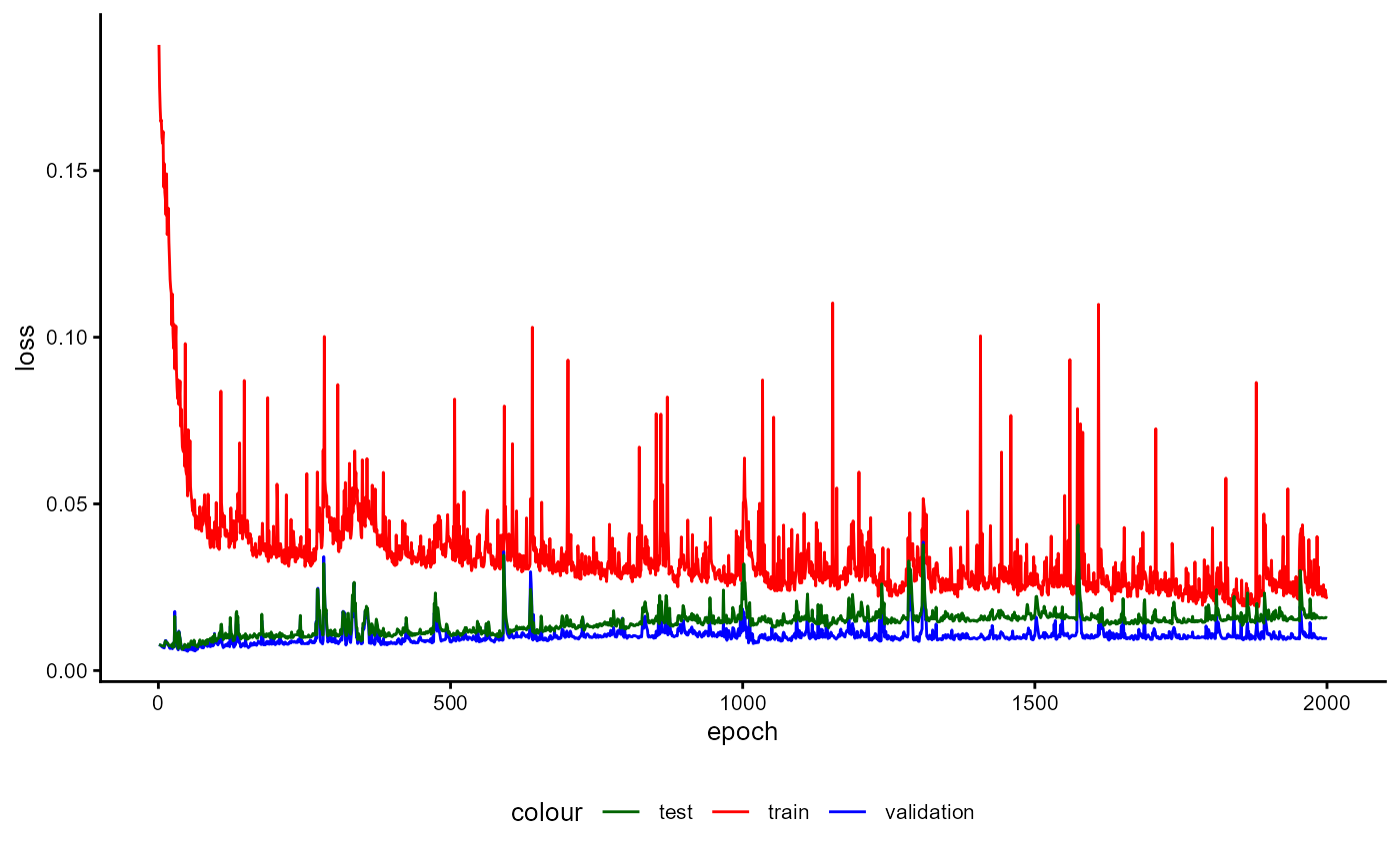
Figure 36: Example of a Training History for a Classifier emphasizing the Loss.
The following plot illustrates how the average iota values developed during the training process.
classifier$plot_training_history(
  final_training = FALSE,
  pl_step = NULL,
  measure = "avg_iota",
  ind_best_model = FALSE,
  ind_selected_model = FALSE,
  x_min = NULL,
  x_max = NULL,
  y_min = NULL,
  y_max = NULL,
  add_min_max = FALSE,
  text_size = 10L
)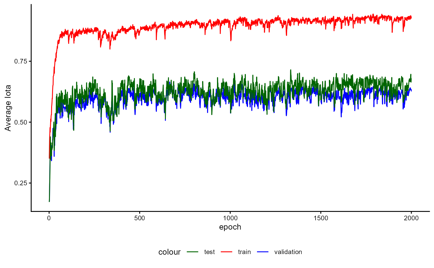
Figure 37: Example of a Training History for a Classifier emphasizing the Average Iota.
Setting ind_best_model to TRUE will display
additional points in the graphic. These points represent the epochs and
their corresponding values according to the chosen metric at which the
model performed best. For metrics such as loss, the values should be
close to 0, while for metrics such as accuracy, balanced accuracy and
average iota, the best values are close to 1. You can see one point for
every fold during training.
classifier$plot_training_history(
  final_training = FALSE,
  pl_step = NULL,
  measure = "loss",
  ind_best_model = TRUE,
  ind_selected_model = FALSE,
  x_min = NULL,
  x_max = NULL,
  y_min = NULL,
  y_max = NULL,
  add_min_max = FALSE,
  text_size = 10L
)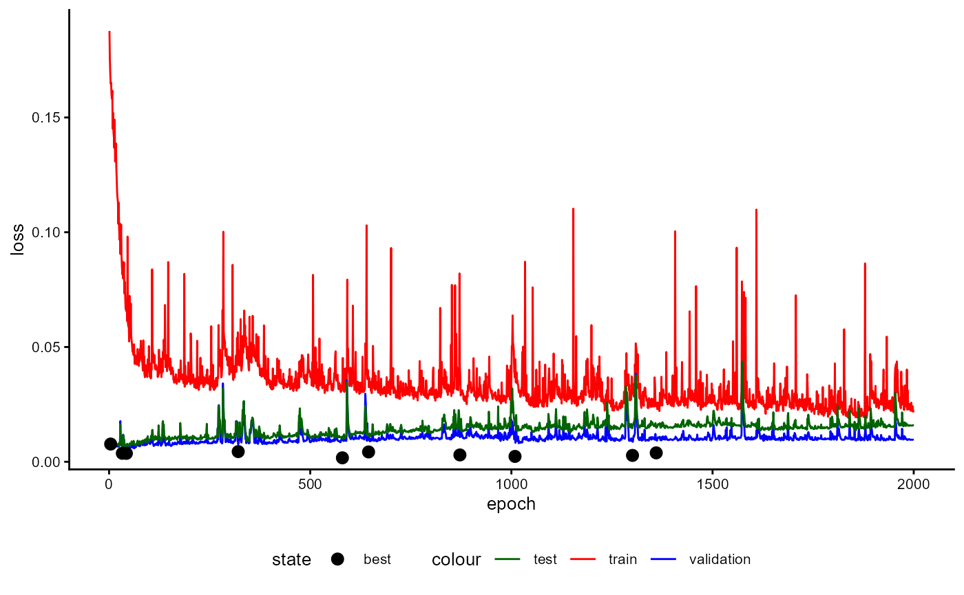
Figure 38: Example of a Training History for a Classifier emphasizing the Loss and the best Model States.
classifier$plot_training_history(
  final_training = FALSE,
  pl_step = NULL,
  measure = "avg_iota",
  ind_best_model = TRUE,
  ind_selected_model = FALSE,
  x_min = NULL,
  x_max = NULL,
  y_min = NULL,
  y_max = NULL,
  add_min_max = FALSE,
  text_size = 10L
)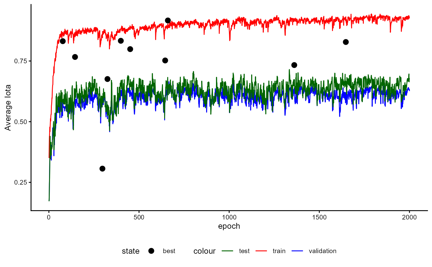
Figure 39: Example of a Training History for a Classifier emphasizing the Average Iota and the best Model States.
Please note that these points indicate the optimal state of the model according to the chosen metric for each fold. However, these values do not necessarily correspond to the final state of the model. This is because the best state of a model during each training loop is determined by the best average iota value. If there are multiple states of a model with the same average iota value, the states with the best average iota value is selected, and then the state with the best balanced accuracy value. If there are still multiple states, the loss is taken into account. In other words, possible best states are all states with the best average iota value. These states are then reduced to those with the best balanced accuracy value, and these states are then reduced again to those with the best loss value. The state with the highest number of epochs is finally used.
Set ind_selected_model to TRUE to add the
final states of the model for every fold.
classifier$plot_training_history(
  final_training = FALSE,
  pl_step = NULL,
  measure = "loss",
  ind_best_model = TRUE,
  ind_selected_model = TRUE,
  x_min = NULL,
  x_max = NULL,
  y_min = NULL,
  y_max = NULL,
  add_min_max = FALSE,
  text_size = 10L
)
Figure 40: Example of a Training History for a Classifier emphasizing the Loss, the best Model States, and the Final Model States.
Since the performance of a model is determined by several factors,
the minimum and maximum values provide a deeper understanding of the
training process. To include these in the plot, set
add_min_max to TRUE. The plot will now show
the full range of values for each epoch according to the chosen
metric.
classifier$plot_training_history(
  final_training = FALSE,
  pl_step = NULL,
  measure = "loss",
  ind_best_model = TRUE,
  ind_selected_model = TRUE,
  x_min = NULL,
  x_max = NULL,
  y_min = NULL,
  y_max = NULL,
  add_min_max = TRUE,
  text_size = 10L
)
Figure 41: Example of a Training History for a Classifier emphasizing the Loss with Minimal and Maximal Values.
Using the argument final_training, you can switch
between the performance estimation stage and the final training stage of
the model. Since the final training phase only differentiates between
training and validation data sets, there is no line for test data. In
addition, there are no folds. Therefore, the argument
add_min_max has no functionality.
classifier$plot_training_history(
  final_training = TRUE,
  pl_step = NULL,
  measure = "loss",
  ind_best_model = TRUE,
  ind_selected_model = TRUE,
  x_min = NULL,
  x_max = NULL,
  y_min = NULL,
  y_max = NULL,
  add_min_max = TRUE,
  text_size = 10L
)
Figure 42: Example of a Training History for a Classifier emphasizing the Loss at the Final Training Phase.
The final important argument is pl_step. This value is
only relevant if the model used pseudo labeling during training. This
parameter allows you to select the step during pseudo labeling that
should be displayed in the plot. This works for performance estimation
as well as the final training stage.
References
Beltagy, I., Peters, M. E., & Cohan, A. (2020). Longformer: The Long-Document Transformer. https://doi.org/10.48550/arXiv.2004.05150
Berding, F., & Pargmann, J. (2022). Iota Reliability Concept of the Second Generation. Berlin: Logos. https://doi.org/10.30819/5581
Berding, F., Riebenbauer, E., Stütz, S., Jahncke, H., Slopinski, A., & Rebmann, K. (2022). Performance and Configuration of Artificial Intelligence in Educational Settings.: Introducing a New Reliability Concept Based on Content Analysis. Frontiers in Education, 1–21. https://doi.org/10.3389/feduc.2022.818365
Boizard, N., Gisserot-Boukhlef, H., Alves, D. M., Martins, A., Hammal, A., Corro, C., Hudelot, C., Malherbe, E., Malaboeuf, E., Jourdan, F., Hautreux, G., Alves, J., El-Haddad, K., Faysse, M., Peyrard, M., Guerreiro, N. M., Fernandes, P., Rei, R. & Colombo, P. (2025). EuroBERT: Scaling Multilingual Encoders for European Languages. https://doi.org/10.48550/arXiv.2503.05500
Campesato, O. (2021). Natural Language Processing Fundamentals for Developers. Mercury Learning & Information. https://ebookcentral.proquest.com/lib/kxp/detail.action?docID=6647713
Cascante-Bonilla, P., Tan, F., Qi, Y. & Ordonez, V. (2020). Curriculum Labeling: Revisiting Pseudo-Labeling for Semi-Supervised Learning. https://doi.org/10.48550/arXiv.2001.06001
Chen, T., Kornblith, S., Norouzi, M. & Hinton, G. (2020). A Simple Framework for Contrastive Learning of Visual Representations. https://doi.org/10.48550/arXiv.2002.05709
Chollet, F., Kalinowski, T., & Allaire, J. J. (2022). Deep learning with R (Second edition). Manning Publications Co. https://learning.oreilly.com/library/view/-/9781633439849/?ar
Conneau, A., Khandelwal, K., Goyal, N., Chaudhary, V., Wenzek, G., Guzmán, F., Grave, E., Ott, M., Zettlemoyer, L., & Stoyanov, V. (2019). Unsupervised Cross-lingual Representation Learning at Scale https://doi.org/10.48550/arXiv.1911.02116
Dai, Z., Lai, G., Yang, Y. & Le, Q. V. (2020). Funnel-Transformer: Filtering out Sequential Redundancy for Efficient Language Processing. https://doi.org/10.48550/arXiv.2006.03236
Devlin, J., Chang, M.‑W., Lee, K., & Toutanova, K. (2019). BERT: Pre-training of Deep Bidirectional Transformers for Language Understanding. In J. Burstein, C. Doran, & T. Solorio (Eds.), Proceedings of the 2019 Conference of the North (pp. 4171–4186). Association for Computational Linguistics. https://doi.org/10.18653/v1/N19-1423
Frochte, J. (2019). Maschinelles Lernen: Grundlagen und Algorithmen in Python (2., aktualisierte Auflage). Hanser.
Ganesh, P., Chen, Y., Lou, X., Khan, M. A., Yang, Y., Sajjad, H., Nakov, P., Chen, D., & Winslett, M. (2021). Compressing Large-Scale Transformer-Based Models: A Case Study on BERT. Transactions of the Association for Computational Linguistics, 9, 1061–1080. https://doi.org/10.1162/tacl_a_00413
Gwet, K. L. (2014). Handbook of inter-rater reliability: The definitive guide to measuring the extent of agreement among raters (Fourth edition). Gaithersburg: STATAXIS.
He, P., Liu, X., Gao, J. & Chen, W. (2020). DeBERTa: Decoding-enhanced BERT with Disentangled Attention. https://doi.org/10.48550/arXiv.2006.03654
He, F., Liu, T. & Tao, D. (2019). Control Batch Size and Learning Rate to Generalize Well: Theoretical and Empirical Evidence. In Advances in neural information processing systems: Bd. 32. 32nd Conference on Neural Information Processing Systems (NeurIPS 2019): Vancouver, Canada, 8-14 December 2019. Curran Associates Inc.
Islam, A., Belhaouari, S. B., Rehman, A. U. & Bensmail, H. (2022). KNNOR: An oversampling technique for imbalanced datasets. Applied Soft Computing, 115, 108288. https://doi.org/10.1016/j.asoc.2021.108288
Jadon, S., & Garg, A. (2020). Hands-On One-shot Learning with Python: Learn to Implement Fast and Accurate Deep Learning Models with Fewer Training Samples Using Pytorch. Packt Publishing Limited. https://ebookcentral.proquest.com/lib/kxp/detail.action?docID=6175328
Kaplan, J., McCandlish, S., Henighan, T., Brown, T. B., Chess, B., Child, R., Gray, S., Radford, A., Wu, J. & Amodei, D. (2020). Scaling Laws for Neural Language Models. https://doi.org/10.48550/arXiv.2001.08361
Kaya, Y. B., & Tantuğ, A. C. (2024). Effect of tokenization granularity for Turkish large language models. Intelligent Systems with Applications, 21, 200335. https://doi.org/10.1016/j.iswa.2024.200335
Keskar, N. S., Mudigere, D., Nocedal, J., Smelyanskiy, M. & Tang, P. T. P. (2017). On Large-Batch Training for Deep Learning: Generalization Gap and Sharp Minima. http://arxiv.org/pdf/1609.04836v2
Krippendorff, K. (2019). Content Analysis: An Introduction to Its Methodology (4th ed.). Los Angeles: SAGE.
Lane, H., Howard, C., & Hapke, H. M. (2019). Natural language processing in action: Understanding, analyzing, and generating text with Python. Shelter Island: Manning.
Larusson, J. A., & White, B. (Eds.). (2014). Learning Analytics: From Research to Practice. New York: Springer. https://doi.org/10.1007/978-1-4614-3305-7
Lee, D.‑H. (2013). Pseudo-Label: The Simple and Efficient Semi-Supervised Learning Method for Deep Neural Networks. CML 2013 Workshop: Challenges in Representation Learning.
Lee-Thorp, J., Ainslie, J., Eckstein, I. & Ontanon, S. (2021). FNet: Mixing Tokens with Fourier Transforms. https://doi.org/10.48550/arXiv.2105.03824
Li, X., Chang, D., Ma, Z., Tan, Z.‑H., Xue, J.‑H., Cao, J., Yu, J. & Guo, J. (2020). OSLNet: Deep Small-Sample Classification With an Orthogonal Softmax Layer. IEEE Transactions on Image Processing, 29, 6482–6495. https://doi.org/10.1109/TIP.2020.2990277
Liu, N. F., Gardner, M., Belinkov, Y., Peters, M. E., & Smith, N. A. (2019). Linguistic Knowledge and Transferability of Contextual Representations. In J. Burstein, C. Doran, & T. Solorio (Eds.), Proceedings of the 2019 Conference of the North (pp. 1073–1094). Association for Computational Linguistics. https://doi.org/10.18653/v1/N19-1112
Liu, Y., Ott, M., Goyal, N., Du, J., Joshi, M., Chen, D., Levy, O., Lewis, M., Zettlemoyer, L., & Stoyanov, V. (2019). RoBERTa: A Robustly Optimized BERT Pretraining Approach. https://doi.org/10.48550/arXiv.1907.11692
Maas, A. L., Daly, R. E., Pham, P. T., Huang, D., Ng, A. Y., & Potts, C. (2011). Learning Word Vectors for Sentiment Analysis. In D. Lin, Y. Matsumoto, & R. Mihalcea (Eds.), Proceedings of the 49th Annual Meeting of the Association for Computational Linguistics: Human Language Technologies (pp. 142–150). Association for Computational Linguistics. https://aclanthology.org/P11-1015
Masters, D. & Luschi, C. (2018). Revisiting Small Batch Training for Deep Neural Networks. https://doi.org/10.48550/arXiv.1804.07612
Meng, Y., Krishnan, J., Wang, S., Wang, Q., Mao, Y., Fang, H., Ghazvininejad, M., Han, J., & Zettlemoyer, L. (2023). Representation Deficiency in Masked Language Modeling. arXiv. https://doi.org/10.48550/ARXIV.2302.02060
Oreshkin, B. N., Rodriguez, P., & Lacoste, A. (2018). TADAM: Task dependent adaptive metric for improved few-shot learning. Advance online publication. https://doi.org/10.48550/arXiv.1805.10123
Papilloud, C., & Hinneburg, A. (2018). Qualitative Textanalyse mit Topic-Modellen: Eine Einführung für Sozialwissenschaftler. Wiesbaden: Springer. https://doi.org/10.1007/978-3-658-21980-2
Pappagari, R., Zelasko, P., Villalba, J., Carmiel, Y., & Dehak, N. (2019). Hierarchical Transformers for Long Document Classification. In 2019 IEEE Automatic Speech Recognition and Understanding Workshop (ASRU) (pp. 838–844). IEEE. https://doi.org/10.1109/ASRU46091.2019.9003958
Pennington, J., Socher, R., & Manning, C. D. (2014). GloVe: Global Vectors for Word Representation. Proceedings of the 2014 Conference on Empirical Methods in Natural Language Processing. https://aclanthology.org/D14-1162.pdf
Ranjan, & Chitta. (2019). Build the right Autoencoder — Tune and Optimize using PCA principles.: Part I. https://towardsdatascience.com/build-the-right-autoencoder-tune-and-optimize-using-pca-principles-part-i-1f01f821999b
Schreier, M. (2012). Qualitative Content Analysis in Practice. Los Angeles: SAGE.
Snell, J., Swersky, K., & Zemel, R. S. (2017). Prototypical Networks for Few-shot Learning. https://doi.org/10.48550/arXiv.1703.05175
Song, K., Tan, X., Qin, T., Lu, J. & Liu, T.‑Y. (2020). MPNet: Masked and Permuted Pre-training for Language Understanding. https://doi.org/10.48550/arXiv.2004.09297
Takeshita, S., Takeshita, Y., Ruffinelli, D. & Ponzetto, S. P. (2025). Randomly Removing 50% of Dimensions in Text Embeddings has Minimal Impact on Retrieval and Classification Tasks. https://doi.org/10.48550/arXiv.2508.17744
Tunstall, L., Werra, L. von, Wolf, T., & Géron, A. (2022). Natural language processing with transformers: Building language applications with hugging face (Revised edition). Heidelberg: O’Reilly.
Vaswani, A., Shazeer, N., Parmar, N., Uszkoreit, J., Jones, L., Gomez, A. N., Kaiser, L., & Polosukhin, I. (2017). Attention Is All You Need. https://doi.org/10.48550/arXiv.1706.03762
Warner, B., Chaffin, A., Clavié, B., Weller, O., Hallström, O., Taghadouini, S., Gallagher, A., Biswas, R., Ladhak, F., Aarsen, T., Cooper, N., Adams, G., Howard, J. & Poli, I. (2024). Smarter, Better, Faster, Longer: A Modern Bidirectional Encoder for Fast, Memory Efficient, and Long Context Finetuning and Inference. https://doi.org/10.48550/arXiv.2412.13663
Wu, Y., Schuster, M., Chen, Z., Le, Q. V., Norouzi, M., Macherey, W., Krikun, M., Cao, Y., Gao, Q., Macherey, K., Klingner, J., Shah, A., Johnson, M., Liu, X., Kaiser, Ł., Gouws, S., Kato, Y., Kudo, T., Kazawa, H., . . . Dean, J. (2016). Google’s Neural Machine Translation System: Bridging the Gap between Human and Machine Translation. https://doi.org/10.48550/arXiv.1609.08144
Zhang, X., Nie, J., Zong, L., Yu, H., & Liang, W. (2019). One Shot Learning with Margin. In Q. Yang, Z.-H. Zhou, Z. Gong, M.-L. Zhang, & S.-J. Huang (Eds.), Lecture Notes in Computer Science. Advances in Knowledge Discovery and Data Mining (Vol. 11440, pp. 305–317). Springer International Publishing. https://doi.org/10.1007/978-3-030-16145-3_24
Zou, L. (2023). Meta-Learning: Theory, Algorithms and Applications. Elsevier Science & Technology. https://ebookcentral.proquest.com/lib/kxp/detail.action?docID=7134465